Numerical simulation of a complex moving rigid body under the impingement of a shock wave in 3D

Abstract

In this paper, we take a numerical simulation of a complex moving rigid body under the impingement of a shock wave in three-dimensional space. Both compressible inviscid fluid and viscous fluid are considered with suitable boundary conditions. We develop a high order numerical boundary treatment for the complex moving geometries based on finite difference methods on fixed Cartesian meshes. The method is an extension of the inverse Lax-Wendroff (ILW) procedure in our works (Cheng et al., Appl Math Mech (Engl Ed) 42: 841–854, 2021; Liu et al.) for 2D problems. Different from the 2D case, the local coordinate rotation in 3D required in the ILW procedure is not unique. We give a theoretical analysis to show that the boundary treatment is independent of the choice of the rotation, ensuring the method is feasible and valid. Both translation and rotation of the body are taken into account in this paper. In particular, we reformulate the material derivative for inviscid fluid on the moving boundary with no-penetration condition, which plays a key role in the proposed algorithm. Numerical simulations on the cylinder and sphere are given, demonstrating the good performance of our numerical boundary treatments.

1 Introduction

In this paper, we design a high order boundary treatment combining high order finite difference scheme for both inviscid and viscous fluids in the 3D time-varying domain. The flow field is between two flat plates parallel to the xz-plane, and there is a rigid body inside it. At the initial moment, there is a plane shock wave perpendicular to the x-axis and moving to the positive direction of the x-axis, towards to the rigid body. Under the impingement of the flow, the rigid body starts to move in the region, then the area of the fluid varies with time, denoted by Ω(t).

In order to prescribe the boundary conditions on the surface of the rigid body, we take the notation Γ(t) to represent the interface between the rigid body and fluid. Hence, we have the boundary of the domain

$$\partial \Omega(t) = \Gamma(t) \cup \Pi_{x} \cup \Pi_{y} \cup \Pi_{z},$$

where, Π_x,Π_y and Π_z are the outer boundaries of the computational area along x-, y- and z-direction, parallel to the yz-, xz- and yz-plane, respectively. Inflow, outflow and reflection boundary conditions are imposed at the left boundary, the right boundary of Π_x and the two boundaries of Π_y, respectively. Notice that, although the physical problem we actually consider is infinite in the z-direction, the domain is truncated in numerical computation. Due to the fact that the rigid body moves in a confined space during a limited period, the area can be assumed to be large enough in the z-direction that the body and the reflective shock waves would not touch Π_z, and then we can impose the outflow boundary conditions on Π_z. Hence, the boundary treatment on Π_z will not affect the computational results of the internal flow field near the rigid boundary. The boundary conditions on the boundary Γ(t) vary with the properties of the fluid. In this paper, we consider both the compressible inviscid fluid and viscous fluid with suitable boundary conditions.

The governing equations for compressible inviscid fluid and viscous fluid in the three-dimensions are written in the same form as follows:

$$ \mathbf{W}_{t}+\mathbf{F}(\mathbf{W})_{x}+\mathbf{G}(\mathbf{W})_{y}+\mathbf{H}(\mathbf{W})_{z}= \frac{\delta}{Re} \left(\mathbf{S_{1}}(\mathbf{W})_{x} + \mathbf{S_{2}}(\mathbf{W})_{y} +\mathbf{S_{3}}(\mathbf{W})_{z} \right), $$

(1)

where (x,y,z)∈Ω(t),W=(ρ,ρu,ρv,ρw,E)^T and

$$ \mathbf{F}(\mathbf{W})=\left(\begin{array}{c}\rho u\\ \rho u^{2}+p\\ \rho uv\\ \rho uw\\u(E+p)\end{array}\right),\quad \mathbf{G}(\mathbf{W})=\left(\begin{array}{c}\rho v\\ \rho uv\\ \rho v^{2}+p\\ \rho vw \\v(E+p)\end{array}\right), \quad \mathbf{H}(\mathbf{W})=\left(\begin{array}{c} \rho w\\ \rho uw\\ \rho vw\\ \rho w^{2}+p\\w(E+p)\end{array}\right). $$

(2)

Here, ρ, u, v, w, p and E stand for density, velocity in x-, y- and z-directions, pressure and total energy per volume, respectively. On the right hand side of (1),

$$\mathbf{S_{1}}(\mathbf{W})= \left(\begin{array}{c} 0\\ \tau_{11}\\ \tau_{21}\\ \tau_{31}\\ \sigma_{1}\\ \end{array}\right),\quad \mathbf{S_{2}}(\mathbf{W})= \left(\begin{array}{c} 0\\ \tau_{12}\\ \tau_{22}\\ \tau_{32}\\ \sigma_{2}\\ \end{array}\right), \quad \mathbf{S_{3}}(\mathbf{W})= \left(\begin{array}{c} 0\\ \tau_{13}\\ \tau_{23}\\ \tau_{33}\\ \sigma_{3}\\ \end{array}\right), $$

with the components of the viscous stress tensor given by

$$ \begin{aligned} & \tau_{11}=\frac{4}{3}u_{x}-\frac{2}{3}v_{y}-\frac{2}{3}w_{z}, \ \ \tau_{22}=\frac{4}{3}v_{y}-\frac{2}{3}u_{x}-\frac{2}{3}w_{z}, \ \ \tau_{33}=\frac{4}{3}w_{z}-\frac{2}{3}u_{x}-\frac{2}{3}v_{y}, \\ & \tau_{12}=\tau_{21}=v_{x}+u_{y}, \quad\quad\,\,\, \tau_{13}=\tau_{31}=u_{z}+w_{x}, \quad\quad\,\,\, \tau_{23}=\tau_{32}=w_{y}+v_{z}, \\ \end{aligned} $$

(3)

and

$$ \begin{aligned} & \sigma_{1} = u\,\tau_{11} + v\,\tau_{12} + w\,\tau_{13} +\frac{(c^{2})_{x}}{(\gamma-1)Pr}, \\ & \sigma_{2} = u\,\tau_{21} + v\,\tau_{22} + w\,\tau_{23} +\frac{(c^{2})_{y}}{(\gamma-1)Pr}, \\ & \sigma_{3} = u\,\tau_{31} + v\,\tau_{32} + w\,\tau_{33} +\frac{(c^{2})_{z}}{(\gamma-1)Pr}. \end{aligned} $$

(4)

Here, Pr is the Prandtl number, Re is the Reynolds number, T=p/ρ is the temperature, and $c=\sqrt {\gamma p/\rho }$ is the sound speed. An equation of state relating the pressure with other variables is given as

$$ p=(\gamma-1)\left(E-\frac{1}{2}\rho\left(u^{2}+v^{2}+w^{2}\right)\right). $$

(5)

γ is the adiabatic constant, which equals to 1.4 for an ideal polytropic gas.

• Compressible inviscid fluid. In this case, δ=0 in the governing Eq. (1) and it becomes the three-dimensional Euler equation,

  $$ \mathbf{W}_{t}+\mathbf{F}(\mathbf{W})_{x}+\mathbf{G}(\mathbf{W})_{y}+\mathbf{H}(\mathbf{W})_{z}= \mathbf{0}, \, $$

  (6)

  The no-penetration boundary conditions are imposed on the boundary of the body surface Γ(t):

  $$ \mathbf{u}\cdot\mathbf{n}=\mathbf{V}_{b}\cdot\mathbf{n}, \quad \forall \, \mathbf{x}\in \Gamma(t), $$

  (7)

  with u=(u,v,w)^T. V_b and n are the velocity and the outward unit normal vector on Γ(t), respectively.

• Compressible viscous fluid. In this case, δ=1 in the governing Eq. (1) and it is the three-dimensional Navier-Stokes (NS) equation,

  $$ \mathbf{W}_{t}+\mathbf{F}(\mathbf{W})_{x}+\mathbf{G}(\mathbf{W})_{y}+\mathbf{H}(\mathbf{W})_{z}= \frac{1}{Re} \left(\mathbf{S_{1}}(\mathbf{W})_{x} + \mathbf{S_{2}}(\mathbf{W})_{y} +\mathbf{S_{3}}(\mathbf{W})_{z} \right), \, $$

  (8)

  On Γ(t), we consider the isothermal no-slip wall boundary condition:

  $$ \left\{ \begin{aligned} &\mathbf{u}=\mathbf{V}_{b}\\ &T=T_{b} \end{aligned} \right. $$

  (9)

  where V_b=(u_b,v_b,w_b)^T and T_b are the velocity and the temperature of the rigid body, respectively.

In this paper, we are trying to numerically solve the partial differential equations (PDEs) (6) and (8) with high order finite difference methods on the fixed Cartesian mesh. Despite the easy generation of the mesh, for such problems there are two main difficulties in numerical simulation:

• A high order finite difference scheme often has a wide stencil, thus we have to evaluate the values at the ghost points near the boundary.

• Another difficulty is that the Cartesian grids intersect with the physical boundary with arbitrary fashion. This often leads to the so-called “cut-cell” problem [1], e.g. in 1D case the first grid is very closed to the physical boundary. If the boundary treatment is not well designed, it may require the time step to be extremely small for the sake of stability and result in the poor computation efficiency. For the moving boundary problems, no matter how the mesh is generated initially, the “cut-cell” problem is unavoidable.

One of the commonly used methods is to generate a body-fitted grid. For simple and fixed boundaries, one may use the smooth mapping between the Cartesian mesh and curvilinear mesh, while this kind of treatment often needs to change the original equations. The new equations can be more complicated than the original equations and also bring additional computation. For the time-varying geometric domain, complex grid management is required at each time step and it may be extremely expensive. Another approach is to use a Cartesian mesh, and take special treatment on the boundaries. There are several numerical boundary treatments listed as follows: embedded boundary method [2–7], immersed boundary method [8–12] and Inverse Lax-Wendroff (ILW) method [13–20], etc.

In this paper, we focus on the ILW boundary treatment for solving the moving boundary problems in 3D. The idea of ILW procedure comes from [21, 22], in which the authors simulated the traffic and pedestrian flow by solving an Eikonal equation at each time step. They used the PDE repeatedly to convert the normal derivative into the tangent derivative at the boundary, and the ghost point values are defined by a Taylor expansion along the normal direction. Enlightened by this approach, Tan and Shu extended it to hyperbolic conservation law equations in [17]. The main idea of the ILW method is to convert the spatial derivative into a time derivative through the PDE, which is in contrast to the traditional Lax-Wendroff scheme, in which the time derivative is converted into spatial derivative (this is exactly the meaning of “inverse”). Numerical results demonstrate that the ILW method can be applied to construct ghost point values when solving equations with high order finite difference methods on a Cartesian mesh in a computational domain with complex geometries. However, the original ILW method proposed in [17] has the following drawbacks:

• Heavy algebra in the ILW procedure for high dimensional nonlinear system.

• For the junction of the inflow and outflow boundary, i.e, the sonic points, the ILW method should be coupled with the least square method to ensure the stability of the scheme.

• The numerical solution obtained by the ILW method cannot satisfy the conservation property while the exact solution of original PDE has this property.

There are several papers to address the issues above. In 2012 Tan et al. proposed the simplified ILW (SILW) method in [19], which greatly reduced the computation cost of the ILW method for solving the system. Ding et al. [14] redefined the concept of conservation for the finite difference scheme, and gave a new ILW method that satisfies the new conservation concept. Lu et al. [16] proposed an ILW method that can deal with the sonic points, which can avoid the situation of the extremely small denominator. Except for hyperbolic conservation laws, the ILW procedure can also be applied to other types of equations. In [23] Filbet and Yang extended the ILW method to handle the Boltzmann equation, and Li et al. studied the ILW procedure for the diffusion problems, and the authors in [15, 24, 25] extended the ILW method to handle the convection-diffusion equation. Stability analyses for both the ILW and the simplified ILW procedures were given in [24–27], in which the authors discussed various situations and gave us the guiding ideology for designing a high order and stable numerical boundary treatment. In particular, theoretical analysis indicates that the carefully designed (S)ILW boundary treatment can maintain stability with the same CFL number (λ_cfl)_max as in the periodic case, ignoring distances of the first grid point to the physical boundary. This means that the SILW method can overcome the “cut-cell" problem.

For moving boundary problems, in [18] Tan and Shu designed an ILW method for inviscid fluid with free-slip no-penetration moving boundary conditions, in which they only considered the translation of the moving boundary. Later, in [13] Cheng et al. reformulated the material derivative and considered both translation and rotation of the body. Recently, [28] extended the moving boundary ILW method to deal with the convection-diffusion equations and simulate the interaction between shock waves and rigid bodies in viscous fluids. In particular, a unified algorithm was given for five cases: pure convection, convection-dominated, convection-diffusion, diffusion-dominated and pure diffusion cases. This paper is an extension of our works [13, 28], in which one and two dimensional moving boundary problems were considered. Now we extend these methods to handle three dimensional problems, with carefully designed numerical boundary conditions such that they can achieve third order of accuracy in smooth case, and no spurious oscillation when there is a shock near the surface. Particularly, in the ILW and SILW procedure, a local coordinate rotation on the boundary point is needed such that the $\hat {x}$-axis of the new coordinate is in the same direction with the outward normal on the boundary. Different from the two dimensional problem, this rotation is not unique. We prove that the rotation will not affect the results via ILW procedure. Hence, the schemes can work with a simple form of rotation. Since the conditions are defined on the moving boundaries, material derivatives are used in the ILW procedure instead of the Eulerian time derivatives. However, this definition of material derivatives for functions limited on the boundaries is not clear. In this paper, we will follow the idea in [13] and reformulate the material derivatives on the moving boundaries with no-penetration condition in 3D.

The organization of the paper is as follows. In Section 2, we introduce the spatial discretization and time evolution method for the Eqs. (6) and (8). In Section 3, we focus on the boundary treatment and present the ILW method in detail. The method of tracking the moving rigid body is discussed in Section 4. Numerical results are given in Section 5 and concluding remarks are given in Section 6.

2 Scheme formulation inside Ω(t)

We assume that the computational domain [x_l,x_r]×[y_l,y_r]×[z_l,z_r] is divided by a Cartesian mesh (x_i,y_j,z_k), and the mesh sizes in each direction are uniform, denoted by Δx,Δy and Δz, respectively,

$$\begin{array}{*{20}l} x_{i}=x_{l}+i \, \Delta x, \quad y_{j}=y_{l}+(j-0.5) \Delta y, \quad z_{k}=z_{l}+k \, \Delta z. \end{array} $$

(10)

Denote W_i,j,k(t) as the approximation to the point value W(x_i,y_j,z_k,t). We will discretize the Eqs. (6) and (8) in the method of lines framework, meaning that the spatial variable is first discretized, then the numerical solution is updated in time by coupling a suitable time integrator.

2.1 Spatial discretization

The semi-discrete approximation of the governing Eq. (1) is given as

$$ {}\frac{d\mathbf{W}_{i,j,k}}{dt} + \frac{\hat{\mathbf{F}}_{i+1/2,j,k}-\hat{\mathbf{F}}_{i-1/2,j,k}}{\Delta x} + \frac{\hat{\mathbf{G}}_{i,j+1/2,k}-\hat{\mathbf{G}}_{i,j-1/2,k}}{\Delta y} + \frac{\hat{\mathbf{H}}_{i,j,k+1/2}-\hat{\mathbf{H}}_{i,j,k-1/2}}{\Delta z} = \mathbf{S}_{i,j,k}, $$

(11)

where $\hat {\mathbf {F}}_{i+1/2,j,k}, \hat {\mathbf {G}}_{i,j+1/2,k}$ and $\hat {\mathbf {H}}_{i,j,k+1/2}$ are numerical fluxes such that the flux difference approximates the derivative to r-th order accuracy,

$$\begin{array}{*{20}l} & \frac{\hat{\mathbf{F}}_{i+1/2,j,k}-\hat{\mathbf{F}}_{i-1/2,j,k}}{\Delta x} = \mathbf{F}(\mathbf{W})_{x}|_{i,j,k} + \mathcal{O} (\Delta x^{r}), \\ & \frac{\hat{\mathbf{G}}_{i,j+1/2,k}-\hat{\mathbf{G}}_{i,j-1/2,k}}{\Delta y} = \mathbf{G}(\mathbf{W})_{y}|_{i,j,k} + \mathcal{O} (\Delta y^{r}), \\ & \frac{\hat{\mathbf{H}}_{i,j,k+1/2}-\hat{\mathbf{H}}_{i,j,k-1/2}}{\Delta z} = \mathbf{H}(\mathbf{W})_{z}|_{i,j,k} + \mathcal{O} (\Delta z^{r}). \end{array} $$

Those numerical fluxes can be obtained by any reasonable finite difference scheme, such as the finite difference (FD) WENO scheme [29], which can achieve high order accuracy in smooth region and avoid numerical oscillatory near discontinuities. Here, we use the third order FD WENO scheme to obtain the numerical fluxes, i.e. r=3. Details are given in Appendix A.

For the Euler Eq. (6), S_i,j,k=0 on the right hand side. And for the NS Eq. (8), S_i,j,k is the approximation to the diffusion terms. Due to the effect of diffusion, we use central finite difference scheme without WENO to obtain S_i,j,k. In particular, the five points central scheme will guarantee fourth order of accuracy, and the formulations for the (mixed) derivatives are given as follows:

$$ \begin{aligned} \frac{\partial f}{\partial x}|_{i,j,k} =& \frac{1}{12\Delta x} (f_{i-2,j,k}-8f_{i-1,j,k}+8f_{i+1,j,k}-f_{i+2,j,k}), \\ \frac{\partial^{2} f}{\partial x^{2}}|_{i,j,k} =& \frac{1}{12\Delta x^{2}} (-f_{i-2,j,k}+16f_{i-1,j,k}-30f_{i,j,k}+16f_{i+1,j,k}-f_{i+2,j,k}), \\ \frac{\partial^{2} f}{\partial x\partial y}|_{i,j,k} =& \frac{1}{144\Delta x \Delta y} ((f_{i-2,j-2,k}-8f_{i-1,j-2,k}+8f_{i+1,j-2,k}-f_{i+2,j-2,k})\\ & -8(f_{i-2,j-1,k}-8f_{i-1,j-1,k}+8f_{i+1,j-1,k}-f_{i+2,j-1,k})\\ & +8(f_{i-2,j+1,k}-8f_{i-1,j+1,k}+8f_{i+1,j+1,k}-f_{i+2,j+1,k})\\ & -(f_{i-2,j+2,k}-8f_{i-1,j+2,k}+8f_{i+1,j-2,k}-f_{i+2,j+2,k})). \end{aligned} $$

(12)

2.2 Time discretization

The semi-discrete scheme (11) is equivalent to the first order ordinary differential equation (ODE) system

$$\begin{array}{*{20}l} \frac{d\mathbf{W}_{i,j,k}}{dt} = \mathcal{L} (\{ \mathbf{W}_{i,j,k} \}), \end{array} $$

(13)

with $\mathcal {L} (\{ \mathbf {W}_{i,j,k} \})$ containing all spatial discritization terms. For time discretization, we use the third-order total variation diminishing (TVD) Runge-Kutta method [30]:

$$ \begin{aligned} \mathbf{W}_{i,j,k}^{(1)}&= \mathbf{W}_{i,j,k}^{n} +\Delta t \mathcal{L}(\{\mathbf{W}_{i,j,k}^{n}\}),\\ \mathbf{W}_{i,j,k}^{(2)}&= \frac{3}{4}\mathbf{W}_{i,j,k}^{n} +\frac{1}{4}\mathbf{W}_{i,j,k}^{(1)}+\frac{1}{4}\Delta t \mathcal{L}(\{\mathbf{W}_{i,j,k}^{(1)}\}),\\ \mathbf{W}_{i,j,k}^{n+1}&= \frac{1}{3}\mathbf{W}_{i,j,k}^{n} +\frac{2}{3}\mathbf{W}_{i,j,k}^{(2)}+\frac{2}{3}\Delta t \mathcal{L}(\{\mathbf{W}_{i,j,k}^{(2)}\}). \end{aligned} $$

(14)

In addition, a following constraint on time step Δt is imposed such that the boundary Γ(t) can move at most one grid in each direction in a time step:

$$ \Delta t \le \min \left(\frac{\Delta x}{V_{b,x,max}}, \frac{\Delta y}{V_{b,y,max}}, \frac{\Delta z}{V_{b,z,max}} \right), $$

(15)

where V_b,x,max,V_b,y,max and V_b,z,max represent the maximum magnitude of the moving velocities in x-, y- and z- directions on the boundary Γ(t).

3 Boundary treatments

In order to make the interior finite difference scheme work, we need to define enough ghost points near the boundaries. Near the outer boundaries Π_x∪Π_y∪Π_z, which consist of straight lines, ghost points are assigned according to the principles of inflow, outflow and reflection boundary conditions. While near the inner boundary Γ(t), we will assign carefully designed values on ghost points. In addition, there is a kind of points called “newly emerging” points that deserve special attention, which are outside the computational domain Ω(t_n−1) at the last time and entering Ω(t_n) at the current time due to the movement of the boundary. In [18], the authors pointed out that the newly emerging points do not need any special treatment, but just set at most one more ghost point in each direction. Then, we can use the same scheme as the interior points to update the values of these points at the last stage of (14). And that is exactly the reason why we give a constraint on the time step in (15).

Note that those ghost points may not lie on the grid. Hence, we follow the idea given in [17] that the method consists of the inverse Lax-Wendroff (ILW) type procedure for inflow boundary conditions and extrapolation for outflow boundary conditions. At the outflow boundary, WENO type extrapolation will be used in case of a shock close to the boundary. And the idea of the ILW procedure is utilizing the PDE repeatedly to write the normal derivatives of the variables W in terms of the time derivatives and tangential derivatives of W, both of which are obtained from boundary conditions. We should note that the boundary location varies with time, hence we will employ the material derivative rather than the Eulerian time derivative on the boundary. In the following subsections, we will concentrate on how to define the values of W_i,j,k at the ghost points.

3.1 Boundary treatment for Euler equations

In the ILW method, we rewrite three-dimensional Euler equations in the form of primitive variables

$$ \mathbf{U}_{t}+\mathbf{A}(\mathbf{U})\mathbf{U}_{x}+\mathbf{B}(\mathbf{U})\mathbf{U}_{y}+\mathbf{C}(\mathbf{U})\mathbf{U}_{z}=\mathbf{0}, $$

(16)

where

$$\mathbf{U}=(\rho, u, v, w,p)^{T},$$

A(U),B(U) and C(U) are Jacobian matrixes, given as

$${}\mathbf{A}(\mathbf{U})= \left(\begin{array}{ccccc}u&\rho &0&0&0\\ 0&u&0&0&\frac{1}{\rho}\\ 0&0&u&0&0\\ 0&0&0&u&0\\ 0&\rho c^{2}&0&0&u\end{array}\right), \, \mathbf{B}(\mathbf{U})=\left(\begin{array}{ccccc}v&0&\rho&0&0\\ 0&v&0&0&0\\ 0&0&v&0&\frac{1}{\rho}\\ 0&0&0&v&0\\ 0&0&\rho c^{2}&0&v\end{array}\right), \, \mathbf{C}(\mathbf{U})=\left(\begin{array}{ccccc}w&0&0&\rho&0\\ 0&w&0&0&0\\ 0&0&w&0&0\\ 0&0&0&w&\frac{1}{\rho}\\ 0&0&0&\rho c^{2}&w\end{array}\right), $$

and $c=\sqrt {\gamma p/\rho }$.

For any ghost point P_i,j,k=(x_i,y_j,z_k), we first find a point P_a=(x_a,y_a,z_a)∈Γ(t) so that its normal vector n outside the rigid body would pass through P_i,j,k:

$$ \left\{\begin{aligned} x_{a}&=x_{c}+r\sin\varphi \, \cos\theta, \\ y_{a}&=y_{c}+r\sin\varphi \, \sin\theta, \\ z_{a}&=z_{c}+r\cos\varphi. \end{aligned}\right. $$

(17)

The normal vector (from fluid to rigid body) of P_a is

$$\mathbf{n} = (-\sin \varphi \, \cos \theta, -\sin \varphi \, \sin \theta, -\cos \varphi).$$

Then, we rotate the coordinate axis locally at P_a such that the $\hat {x}$-axis of the new coordinate system is in the same direction with n. We want to remark the fact that the rotation is not unique due to $\hat {y}$- and $\hat {z}$-axis can be any orthogonal vectors in the tangent plane with respect to the rigid body at P_a, but it will not effect the results via ILW procedure. Particularly, in Appendix B, we prove the following theorem:

Theorem 1

The ILW boundary procedure for the Euler equation is independent of the choice of the rotation, i.e, we can get the same boundary scheme even with different choices of rotation.

Therefore, we can get the same formulation even with different choices of tangent vectors. Here, we give one of these rotation methods and apply it to our later computation. The new local coordinate system $(\hat {x}, \hat {y}, \hat {z})$ and the coordinate transformation matrix T are given as

$$ \left(\begin{array}{c}\hat{x}\\ \hat{y}\\ \hat{z}\end{array}\right)=\mathbf{T}\left(\begin{array}{c}x\\ y\\ z\end{array}\right), \quad \text{and} \quad \mathbf{T} =\left(\begin{array}{ccc} -\cos \theta \cdot \sin \varphi & -\sin \theta \cdot \sin \varphi & -\cos \varphi \\ \sin \theta & -\cos \theta & 0 \\ -\cos \theta \cdot \cos \varphi & -\cos \varphi \cdot \sin \theta & \sin \varphi \\ \end{array} \right). $$

(18)

Consequently, we can prove that the Euler Eq. (16) has the same form in the new coordinate system as those in the original coordinate system:

$$ \hat{\mathbf{U}}_{t}+\mathbf{A}(\hat{\mathbf{U}})\hat{\mathbf{U}}_{\hat{x}}+\mathbf{B}(\hat{\mathbf{U}})\hat{\mathbf{U}}_{\hat{y}}+\mathbf{C}(\hat{\mathbf{U}})\hat{\mathbf{U}}_{\hat{z}}=\mathbf{0}, $$

(19)

with

$$\begin{array}{*{20}l} \hat{\mathbf{U}}=(\rho,\hat{u},\hat{v},\hat{w},p)^{T}, \quad \text{and} \quad \left(\begin{array}{c}\hat{u}\\ \hat{v}\\ \hat{w}\end{array}\right)=\mathbf{T}\left(\begin{array}{c}u\\ v\\ w\end{array}\right). \end{array} $$

(20)

Next, we can approximate the values $\hat {\mathbf {U}}_{i,j,k}$ at point P_i,j,k by a Taylor expansion at point P_a. For instance, a third order approximation is given as

$$ \hat{\mathbf{U}}_{ijk} = \hat{\mathbf{U}}_{a} +(\mathbf{r} \cdot \mathbf{n})\hat{\mathbf{U}}_{a}^{(1)} + \frac{1}{2}(\mathbf{r} \cdot \mathbf{n})^{2} \,\hat{\mathbf{U}}_{a}^{(2)}, $$

(21)

where r is a vector going from P_a to $P_{i,j,k}, \hat {\mathbf {U}}_{a}$ (or $\hat {\mathbf {U}}^{(0)}_{a}$) is the point value at P_a, and $\hat {\mathbf {U}}_{a}^{(1)}$ and $\hat {\mathbf {U}}_{a}^{(2)}$ are the normal derivatives $\hat {\mathbf {U}}_{\hat {x}}|_{P_{a}}$ and $\hat {\mathbf {U}}_{\hat {x}\hat {x}}|_{P_{a}}$, respectively. It can be extended to arbitrary high order accuracy easily by keeping more terms in the Taylor expansion. For the current third-order scheme, we just need to get the values $\hat {\mathbf {U}}_{a}^{(m)}, m=0, 1, 2$.

Before that, a local characteristic decomposition should be done at P_a, with the eigen-decomposition

$$\mathbf{A}(\hat{\mathbf{U}}_{a})=\mathbf{L}^{-1}_{a}\mathbf{\Lambda}_{a} \mathbf{L}_{a},$$

where, Λ is the diagonal matrix consisting of the eigenvalues of $\mathbf {A}(\hat {\mathbf {U}})$, and L forms from the corresponding left eigenvectors {l₁,…,l₅}:

$$\begin{array}{*{20}l} \mathbf{L}_{a} = (\mathbf{l}_{1},\ldots, \mathbf{l}_{5})^{T} = \left(\begin{array}{cccc} l_{1,1} & l_{1,2} & \cdots & l_{1,5} \\ l_{2,1} & l_{2,2} & \cdots & l_{2,5} \\ \vdots & \vdots & \ddots & \vdots \\ l_{5,1} & l_{5,2} & \cdots & l_{5,5} \\ \end{array}\right). \end{array} $$

Notice that the point value $\hat {\mathbf {U}}_{a}$ is unknown, we will use the WENO extrapolation to obtain the approximation $\hat {\mathbf {U}}_{a}^{ext}$ (see Appendix C) and then substitute it into the formulations above, obtaining $\mathbf {L}_{a}=\mathbf {L}(\hat {\mathbf {U}}_{a}^{ext})$. After that, convert the original variables $\hat {\mathbf {U}}$ to the characteristic fields $\mathbf {V}=\mathbf {L}_{a}\hat {\mathbf {U}}$. Since the eigenvalues of $\mathbf {A}(\hat {\mathbf {U}})$ are

$$\hat{u}-c, \, \hat{u}, \, \hat{u}, \, \hat{u}, \, \hat{u}+c,$$

the moving speeds of five characteristic lines relative to the boundary normal direction are −c, 0, 0, 0, c, respectively.

3.1.1 Reformulation of the material derivative in 3D

In the ILW procedure, we convert normal spatial derivatives to tangential and time derivatives of the given boundary condition using the PDE. Specifically, for moving boundaries, we would employ the material derivatives of the boundary conditions. Details will be shown in Section 3.1.2. For any function $\tilde {g}\in C^{1}(\mathbb {R}^{3}\times \mathbb {R}^{+})$, the material derivative is given as

$$\begin{array}{*{20}l} \frac{D\tilde{g}}{Dt}= \frac{\partial \tilde{g}}{\partial t} + u \frac{\partial \tilde{g}}{\partial x} + v \frac{\partial \tilde{g}}{\partial y} + w \frac{\partial \tilde{g}}{\partial z}, \end{array} $$

(22)

where, (u,v,w) is the flow velocity. Unfortunately, the definition above can not be used for the functions defined on boundary only, such as the normal vector, since the spatial derivatives may not exist. Therefore, for the functions limited on the surface in three-dimensional space, we will give a new definition of material derivative, which would play a key role in the ILW method in the following subsection.

Suppose that the three-dimensional moving boundary Γ(t) is given as

$$\mathbf{X}_{b} = (x(\tau_{1},\tau_{2},t), y(\tau_{1},\tau_{2},t), z(\tau_{1},\tau_{2},t)), $$

where (τ₁,τ₂) are parameters in [τ₁₀,τ₁₁]×[τ₂₀,τ₂₁]. For example, the surface of a unit sphere in 3D can be described in spherical coordinates:

$$x=\sin(\tau_{1}) \cos(\tau_{2}), \quad y=\sin(\tau_{1}) \sin(\tau_{2}), \quad z=\cos(\tau_{2}), $$

where, (τ₁,τ₂) are parameters in [0,2π]×[−π/2,π/2].

Assume that, the parametric equation Γ(t) is regular, i.e., $\frac {\partial \mathbf {X}_{b}}{\partial \tau _{1}}$ and $\frac {\partial \mathbf {X}_{b}}{\partial \tau _{2}}$ are linearly independent. Thus, $\frac {\partial \mathbf {X}_{b}}{\partial \tau _{1}}, \frac {\partial \mathbf {X}_{b}}{\partial \tau _{2}}$ and n form a basis of the three-dimensional space. Then, the velocities of the fluid and the boundary can be written as follows:

$$ \begin{aligned} & \mathbf{u}=u_{n}\, \mathbf{n}+u_{\tau_{1}}\frac{\partial \mathbf{X}_{b}}{\partial\tau_{1}}+u_{\tau_{2}}\frac{\partial \mathbf{X}_{b}}{\partial\tau_{2}}, \\ & \mathbf{V}_{b}=V_{b,n}\,\mathbf{n} + V_{b,\tau_{1}}\frac{\partial \mathbf{X}_{b}}{\partial\tau_{1}} + V_{b,\tau_{2}}\frac{\partial \mathbf{X}_{b}}{\partial\tau_{2}}. \end{aligned} $$

(23)

Definition 1

Suppose there is a function defined on Γ(t): $g(\tau _{1},\tau _{2},t)\in C^{1}([\tau _{10},\tau _{11}]\times [\tau _{20},\tau _{21}]\times \mathbb {R}^{+})$. The material derivative is defined as:

$$ L(g) = \frac{\partial g}{\partial t} + (u_{\tau_{1}}-V_{b,\tau_{1}})\frac{\partial g}{\partial \tau_{1}} + (u_{\tau_{2}}-V_{b,\tau_{2}})\frac{\partial g}{\partial \tau_{2}}. $$

(24)

Moreover, it has the following property, which indicates the equivalence between our new definition (24) and the traditional definition of material derivative on no-penetration boundary.

Theorem 2

Suppose Γ(t)=(x(τ₁,τ₂,t),y(τ₁,τ₂,t),z(τ₁,τ₂,t)) is a smooth surface in three dimensions, and the no-penetration boundary condition holds on Γ(t), i.e. u·n=V_b·n. For any $\tilde {g}(x,y,z,t)\in C^{1}(\mathbb {R}^{3}\times \mathbb {R}^{+})$, we can define a function g on Γ(t):

$$ g(\tau_{1},\tau_{2},t)=\tilde{g}(x(\tau_{1},\tau_{2},t),y(\tau_{1},\tau_{2},t),z(\tau_{1},\tau_{2},t),t). $$

(25)

Then the following equation is true:

$$ L(g)=\frac{D\tilde{g}}{Dt}=\frac{\partial \tilde{g}}{\partial t}+\nabla \tilde{g}\cdot\mathbf{u}, $$

(26)

where $\frac {D}{Dt}$ is the material derivative given in (22).

Proof According to the formula (23) and u·n=V_b·n, we know that u_n=V_b,n. Using the chain rule, we can obtain that

$$\begin{aligned} & \frac{\partial g}{\partial t}=\frac{\partial \tilde{g}}{\partial t}+\frac{\partial \tilde{g}}{\partial x}\frac{\partial x}{\partial t} +\frac{\partial \tilde{g}}{\partial y}\frac{\partial y}{\partial t}+\frac{\partial \tilde{g}}{\partial z}\frac{\partial z}{\partial t} =\frac{\partial \tilde{g}}{\partial t}+\nabla \tilde{g}\cdot\mathbf{V}_{b}, \\ & \frac{\partial g}{\partial \tau_{1}}=\frac{\partial \tilde{g}}{\partial x}\frac{\partial x}{\partial \tau_{1}} +\frac{\partial \tilde{g}}{\partial y}\frac{\partial y}{\partial \tau_{1}}+\frac{\partial \tilde{g}}{\partial z}\frac{\partial z}{\partial \tau_{1}} =\nabla \tilde{g}\cdot\frac{\partial \mathbf{X}_{b}}{\partial \tau_{1}}, \\ & \frac{\partial g}{\partial \tau_{2}}=\frac{\partial \tilde{g}}{\partial x}\frac{\partial x}{\partial \tau_{2}} +\frac{\partial \tilde{g}}{\partial y}\frac{\partial y}{\partial \tau_{2}}+\frac{\partial \tilde{g}}{\partial z}\frac{\partial z}{\partial \tau_{2}} =\nabla \tilde{g}\cdot\frac{\partial \mathbf{X}_{b}}{\partial \tau_{2}}. \end{aligned} $$

Therefore,

$$\begin{array}{*{20}l} L(g) =&\frac{\partial g}{\partial t} + (u_{\tau_{1}}-V_{b,\tau_{1}})\frac{\partial g}{\partial \tau_{1}} + (u_{\tau_{2}}-V_{b,\tau_{2}})\frac{\partial g}{\partial \tau_{2}}\\ =&\frac{\partial \tilde{g}}{\partial t}+\nabla \tilde{g}\cdot\mathbf{V}_{b}+(u_{\tau_{1}}-V_{b,\tau_{1}})\nabla \tilde{g}\cdot\frac{\partial \mathbf{X}_{b}}{\partial \tau_{1}}\\ &+(u_{\tau_{2}}-V_{b,\tau_{2}})\nabla \tilde{g}\cdot\frac{\partial \mathbf{X}_{b}}{\partial \tau_{2}}+(u_{n}-V_{b,n})\nabla \tilde{g}\cdot\mathbf{n}\\ =&\frac{\partial \tilde{g}}{\partial t}+\nabla \tilde{g}\cdot\mathbf{u} =\frac{D\tilde{g}}{Dt}. \end{array} $$

This completes the proof.

In the next subsection, we will use the definition L (24) on the given boundary conditions in the ILW process. For easy notation, we write L(g) as $\frac {Dg}{Dt}$ in the following subsections.

3.1.2 ILW method

With the boundary conditions and the material derivative given in Definition 1, we now proceed to construct $\hat {\mathbf {U}}^{(m)}_{a} = ((\hat {U}_{1})^{(m)}_{a}, \ldots, (\hat {U}_{5})^{(m)}_{a})^{T}, m=0,1,2$.

• At first, we want to find the value of $\hat {\mathbf {U}}^{(0)}_{a}$. The no-penetration condition $\hat {u} = \hat {\mathbf {u}} \cdot \mathbf {n} = \mathbf {V}_{b}\cdot \mathbf {n}$ can be rewritten as

  $$(\hat{U}_{2})^{(0)}_{a} = \mathbf{V}_{b}\cdot \mathbf{n}.$$

  Do the extrapolation of those outgoing characteristic variables, and we have the following equations

  $$\mathbf{l}_{j} \cdot \hat{\mathbf{U}}^{(0)}_{a} = (V_{j})^{(0)}_{a}, \quad j=2,\ldots,5, $$

  where, $(V_{j})_{a}^{(0)}$ are obtained by the WENO extrapolation. Hence, those equations tell us a system as

  $$ \left(\begin{array}{ccccc}0&1&0&0&0\\ l_{2,1} & l_{2,2} & l_{2,3} & l_{2,4} & l_{2,5} \\ l_{3,1} & l_{3,2} & l_{3,3} & l_{3,4} & l_{3,5} \\ l_{4,1} & l_{4,2} & l_{4,3} & l_{4,4} & l_{4,5} \\ l_{5,1} & l_{5,2} & l_{5,3} & l_{5,4} & l_{5,5} \\ \end{array}\right) \left(\begin{array}{c} (\hat{U}_{1})^{(0)}_{a} \\ (\hat{U}_{2})^{(0)}_{a} \\ (\hat{U}_{3})^{(0)}_{a} \\ (\hat{U}_{4})^{(0)}_{a} \\ (\hat{U}_{5})^{(0)}_{a} \end{array}\right) = \left(\begin{array}{c}\mathbf{V}_{b}\cdot \mathbf{n} \\ (V_{2})_{a}^{(0)} \\ (V_{3})_{a}^{(0)} \\ (V_{4})_{a}^{(0)} \\ (V_{5})_{a}^{(0)} \\ \end{array}\right). $$

  (27)

  Thus, $\hat {\mathbf {U}}^{(0)}_{a}$ can be obtained by solving the above system.

• Then, we want to find the derivative of $\hat {\mathbf {U}}^{(1)}_{a}$. From the second equation of Euler equations with primitive variables we can get

  $$p_{\hat{x}}=-\rho\frac{D\hat{u}}{Dt}=\rho\left[\hat{\mathbf{u}}\cdot\frac{D\hat{\mathbf{n}}}{Dt}-\frac{D}{Dt}(\mathbf{V}_{b}\cdot\mathbf{n})\right],$$

  where

  $$\begin{aligned} & \frac{D\mathbf{n}}{Dt}=\frac{\mathbf{u}-\mathbf{V}_{b}}{r},\qquad \frac{D\hat{\mathbf{n}}}{Dt}=\mathbf{T}\frac{D\mathbf{n}}{Dt}, \\ & \frac{D}{Dt}(\mathbf{V}_{b}(t)\cdot\mathbf{n}) = \frac{d\mathbf{V}_{b}}{dt}\cdot \mathbf{n} + \mathbf{V}_{b}\cdot\frac{D\mathbf{n}}{Dt}. \end{aligned} $$

  So we get $\hat {\mathbf {U}}^{(1)}_{a}$ by solving the following system:

  $$ \left\{ \begin{aligned} & (\hat{U}_{5})^{(1)}_{a} = \rho\left(\hat{\mathbf{u}}\cdot\frac{D\hat{\mathbf{n}}}{Dt}-\frac{d}{dt}(\mathbf{V}_{b}\cdot\mathbf{n})\right), \\ & \mathbf{l}_{j} \cdot \hat{\mathbf{U}}^{(1)}_{a} = (V_{j})^{(1)}_{a}, \qquad j=2,\ldots,5, \end{aligned} \right. $$

  (28)

  Again, $(V_{j})_{a}^{(1)}$ are obtained by the WENO extrapolation.

• Finally, for the second derivative $\hat {\mathbf {U}}^{(2)}_{a}$, we will employ the idea of simplified ILW (SILW) procedure proposed in [20], and the second derivative can be obtained by WENO extrapolation.

Once $\hat {\mathbf {U}}^{(m)}_{a}, m=0, 1, 2$ are obtained, we can use (21) to get $\hat {\mathbf {U}}_{i,j,k}$, and further U_i,j,k and W_i,j,k.

3.1.3 Coupling with RK time discretization

Notice that the numerical method we have described previously is for time level t_n only. When coupling with the third order RK scheme (14), we need to match the time levels when constructing values of ghost points in the two intermediate stages W⁽¹⁾ and W⁽²⁾. In particular, the velocity $\hat {u}$ at the boundary at each RK stage is necessary as the boundary condition, and we need to update $\hat {u}$ with the following formulations instead of the RK scheme (14) to maintain the third order in time:

$$ \begin{aligned} & \hat{u}^{(1)} = \hat{u}^{n} + \Delta t \frac{\partial \hat{u}}{\partial t} |_{\mathbf{x}=\mathbf{X}_{b}(t_{n}), t =t_{n}}, \\ & \hat{u}^{(2)} = \hat{u}^{n} + \frac{\Delta t}{2}\frac{\partial \hat{u}}{\partial t} |_{\mathbf{x}=\mathbf{X}_{b}(t_{n}), t =t_{n}} + \frac{\Delta t^{2}}{4} \frac{\partial^{2} \hat{u}}{\partial t^{2}} |_{\mathbf{x}=\mathbf{X}_{b}(t_{n}), t =t_{n}}. \end{aligned} $$

(29)

As in [18], we can use a standard Lax-Wendroff procedure to get the time derivatives as we want. More specifically, employing the second equation of (16) repeatedly, we can get the time derivatives $\frac {\partial \hat {u}}{\partial t}$ and $\frac {\partial ^{2} \hat {u}}{\partial t^{2}}$ in terms of spatial derivatives. After finishing an inverse Lax Wendroff procedure at the time level t_n, all the first and second order spatial derivatives values at x=X_b(t_n) are given. Hence, we can get $\frac {\partial \hat {u}}{\partial t}|_{\mathbf {x}=\mathbf {X}_{b}(t_{n}), t=t_{n}}$ and $\frac {\partial ^{2} \hat {u}}{\partial t^{2}}|_{\mathbf {x}=\mathbf {X}_{b}(t_{n}), t=t_{n}}$ with these spatial derivatives. More details can be found in [18].

3.2 Boundary treatments for NS equation

Similar to the case in Section 3.1, to define the value at a ghost point P_i,j,k=(x_i,y_j,z_k), we set up a local coordinate system at P_a by (18) at first. Then, consider the variables and system in the local coordinate system. Again, the rotation is not unique but will not affect the results of boundary scheme. The proof is very similar to the Euler equation in Appendix B. We will not repeat it here.

Due to the fact that the Dirichlet boundary conditions are given for velocity $\hat {\mathbf {U}}$ and temperature T, we rewrite the Eq. (8) with respect to the new variables

$$\hat{\mathbf{U}}=(\rho, \hat{u}, \hat{v}, \hat{w}, T)^{T},$$

and then,

$$ \hat{\mathbf{U}}_{t} + \mathbf{D}(\hat{\mathbf{U}})\hat{\mathbf{U}}_{\hat{x}} = \mathbf{E}(\hat{\mathbf{U}})\hat{\mathbf{U}}_{\hat{x}\hat{x}} + \mathbf{Res}, $$

(30)

The matrixes and source term are given as

$$ \mathbf{D}(\hat{\mathbf{U}}) = \left(\begin{array}{ccccc} \hat{u}&\rho&0&0&0\\ \frac{T}{\rho}&\hat{u}&0&0&1\\ 0&0&\hat{u}&0&0\\ 0&0&0&\hat{u}&0\\ 0&(\gamma-1)T&0&0&\hat{u} \end{array}\right), \quad \mathbf{E}(\hat{\mathbf{U}}) = \left(\begin{array}{ccccc} 0&0&0&0&0\\ 0&\frac{4}{3Re\cdot\rho}&0&0&0\\ 0&0&\frac{1}{Re\cdot\rho}&0&0\\ 0&0&0&\frac{1}{Re\cdot\rho}&0\\ 0&0&0&0&\frac{\gamma}{Pr \cdot Re\cdot \rho} \end{array}\right), $$

(31)

and

$$ \mathbf{Res}=\left(\begin{array}{c} {Res}_{1}\\ {Res}_{2}\\ {Res}_{3}\\ {Res}_{4}\\ {Res}_{5}\\ \end{array}\right) =\left(\begin{array}{c} -\rho(\hat{v}_{\hat{y}}+\hat{w}_{\hat{z}})-\hat{v}\rho_{\hat{y}}-\hat{w}\rho_{\hat{z}}\\ \frac{1}{Re\cdot \rho}(\hat{u}_{\hat{y}\hat{y}}+\hat{u}_{\hat{z}\hat{z}}+\frac{1}{3}\hat{v}_{\hat{x}\hat{y}}+\frac{1}{3}\hat{w}_{\hat{x}\hat{z}})-\hat{v}{\hat{u}}_{\hat{y}}-\hat{w}{\hat{u}}_{\hat{z}}\\ \frac{1}{Re\cdot \rho}(\frac{4}{3}\hat{v}_{\hat{y}\hat{y}}+\hat{v}_{\hat{z}\hat{z}}+\frac{1}{3}\hat{u}_{\hat{x}\hat{y}}+\frac{1}{3}\hat{w}_{\hat{y}\hat{z}})-\frac{1}{\rho}P_{\hat{y}}-\hat{v}{\hat{v}}_{\hat{y}}-\hat{w}{\hat{v}}_{\hat{z}}\\ \frac{1}{Re\cdot \rho}(\hat{w}_{\hat{y}\hat{y}}+\frac{4}{3}\hat{w}_{\hat{z}\hat{z}}+\frac{1}{3}\hat{u}_{\hat{x}\hat{z}}+\frac{1}{3}\hat{v}_{\hat{y}\hat{z}})-\frac{1}{\rho}P_{\hat{z}}-\hat{v}{\hat{w}}_{\hat{y}}-\hat{w}{\hat{w}}_{\hat{z}}\\ \frac{\gamma}{Re\cdot \rho \cdot Pr}(T_{\hat{y}\hat{y}}+T_{\hat{z}\hat{z}})+NLT \\ \end{array}\right), $$

(32)

with

$$ \begin{aligned} NLT= \frac{\gamma-1}{Re\cdot \rho} \left(-\frac{2}{3}(\hat{u}_{\hat{x}}+\hat{v}_{\hat{y}}+\hat{w}_{\hat{z}})^{2} +2(\hat{u}_{\hat{x}}^{2}+\hat{v}_{\hat{y}}^{2}+\hat{w}_{\hat{z}}^{2}) +2(\hat{v}_{\hat{x}}+\hat{u}_{\hat{y}})^{2} \right. \\ \left. +2(\hat{w}_{\hat{x}} +\hat{u}_{\hat{z}})^{2} +2(\hat{v}_{\hat{z}}+\hat{w}_{\hat{y}})^{2} \right). \end{aligned} $$

(33)

Again, the values $\hat {\mathbf {U}}_{i,j,k}$ at point P_i,j,k will be approximated by a Taylor expansion in $\hat {x}$-direction at point P_a. Once obtaining the point value $\hat {\mathbf {U}}_{a}$, and normal derivatives $\hat {\mathbf {U}}^{(1)}_{a}$ and $\hat {\mathbf {U}}^{(2)}_{a}$, we can get the third order approximation of $\hat {\mathbf {U}}_{i,j,k}$ via (21).

Note that in the boundary treatment for the Euler equations in Section 3.1, the boundary values $\hat {\mathbf {U}}_{a}^{(m)}$ are obtained via either the ILW method based on the boundary conditions or the extrapolation of the outgoing variables. However, for the compressible NS equation, totally different boundary treatments are needed for the diffusion-dominated and the convection-dominated regimes. Hence, [28] designed the numerical methods based on a careful combination of the boundary treatments for the two regimes and obtained a stable and accurate boundary condition for general convection-diffusion equations with either still or moving boundaries. Here, we extend the numerical method to our 3D model with the given isothermal no-slip wall boundary condition.

3.2.1 The material derivative in 3D

For the NS equation with moving boundary, the material derivative is also necessary in the ILW method.

$$\frac{D\hat{\mathbf{U}}}{Dt} = \hat{\mathbf{U}}_{t} + \hat{u} \, \hat{\mathbf{U}}_{\hat{x}} + \hat{v} \, \hat{\mathbf{U}}_{\hat{y}} + \hat{w} \, \hat{\mathbf{U}}_{\hat{z}}. $$

For the no-slip boundary, the material derivatives for the boundary and fluid are the same,

$$\frac{D \hat{\mathbf{U}}}{Dt} = \frac{D \hat{\mathbf{U}}_{b}}{Dt}. $$

Moreover, since T_b is constant, hence DT_b/Dt=0. And $D\hat {\mathbf {u}}/D t = d\mathbf {V}_{b}/dt$ equal to the acceleration of the rigid body. As a consequence,

$$ \left\{ \begin{aligned} &\frac{D\rho}{Dt} + \rho(\hat{u}_{\hat{x}}+\hat{v}_{\hat{y}}+\hat{w}_{\hat{z}}) = 0\\ &\frac{D\hat{u}}{Dt}+\frac{1}{\rho}p_{\hat{x}} =\frac{1}{Re\rho}(\frac{4}{3}\hat{u}_{\hat{x}\hat{x}}+\hat{u}_{\hat{y}\hat{y}}+\hat{u}_{\hat{z}\hat{z}}+\frac{1}{3}\hat{v}_{\hat{x}\hat{y}}+\frac{1}{3}\hat{w}_{\hat{x}\hat{z}})\\ &\frac{D\hat{v}}{Dt}+\frac{1}{\rho}p_{\hat{y}} =\frac{1}{Re\rho}(\hat{v}_{\hat{x}\hat{x}}+\frac{4}{3}\hat{v}_{\hat{y}\hat{y}}+\hat{v}_{\hat{z}\hat{z}}+\frac{1}{3}\hat{u}_{\hat{x}\hat{y}}+\frac{1}{3}\hat{w}_{\hat{y}\hat{z}})\\ &\frac{D\hat{w}}{Dt}+\frac{1}{\rho}p_{\hat{z}} =\frac{1}{Re\rho}(\hat{w}_{\hat{x}\hat{x}}+\hat{w}_{\hat{y}\hat{y}}+\frac{4}{3}\hat{w}_{\hat{z}\hat{z}}+\frac{1}{3}\hat{u}_{\hat{x}\hat{z}}+\frac{1}{3}\hat{v}_{\hat{y}\hat{z}})\\ &\frac{DT}{Dt}+(\gamma-1)T(\hat{u}_{\hat{x}}+\hat{v}_{\hat{y}}+\hat{w}_{\hat{z}})=\frac{\gamma}{\rho\,Re\, Pr}(T_{\hat{x}\hat{x}}+T_{\hat{y}\hat{y}}+T_{\hat{z}\hat{z}})+NLT\\ \end{aligned} \right. $$

(34)

3.2.2 ILW method

In particular, the derivatives $\hat {\mathbf {U}}_{a}^{(m)}, m=1, 2$, are a combination of those derived from the ILW procedure and the extrapolation procedure from interior points. For easy notation, we use the subscript “ilw" and “ext" to denote derivatives $\hat {\mathbf {U}}_{a}^{(m)}$ obtained through the ILW procedure $\hat {\mathbf {U}}^{(m)}_{a,ilw}$ and the extrapolation $\hat {\mathbf {U}}^{(m)}_{a,ext}$, respectively.

Here, the matrix $\mathbf {D}(\hat {\mathbf {U}})$ is also diagonalizable,

$$\mathbf{D}(\hat{\mathbf{U}})=\mathbf{L}^{-1}(\hat{\mathbf{U}})\mathbf{\Lambda} (\hat{\mathbf{U}})\mathbf{L}(\hat{\mathbf{U}}), $$

with $\mathbf {\Lambda } (\hat {\mathbf {U}}) = diag\{ \hat {u}-c, \hat {u}, \hat {u}, \hat {u}, \hat {u}+c\}$. Hence, considering the characteristic variables $\mathbf {V}=\mathbf {L}_{a}\hat {\mathbf {U}}$, the components V₂,⋯,V₅ are the outflow variables, and V₁ is the inflow variable. Again, $\hat {\mathbf {U}}_{a}^{ext}$ is used in the characteristic decomposition.

• Construct the point value $\hat {\mathbf {U}}_{a}^{(0)}$. Note that the boundary condition (9) gives the value of $\hat {\mathbf {U}}$ and T at the boundary Γ(t) directly, so we can set

  $$ (\hat{U}_{2})_{a}^{(0)}=\hat{u}_{b}, \quad (\hat{U}_{3})_{a}^{(0)}=\hat{v}_{b}, \quad (\hat{U}_{4})_{a}^{(0)}=\hat{w}_{b}, \quad (\hat{U}_{5})_{a}^{(0)}=T_{b}. $$

  (35)

  Since V₅ is the outgoing variable, we have the relation that

  $$\begin{array}{*{20}l} \mathbf{l}_{5} \cdot \hat{\mathbf{U}}_{a}^{(0)} = V_{5} = \mathbf{l}_{5} \cdot \hat{\mathbf{U}}^{(0)}_{a,ext}. \end{array} $$

  Therefore, we can obtain the value of $(\hat {U}_{1})_{a}^{(0)}$ as follows,

  $$ (\hat{U}_{1})_{a}^{(0)} = \frac{(\hat{U}_{1})^{(0)}_{a,ext}}{ (\hat{U}_{5})^{(0)}_{a,ext}} \, \left(2\,(\hat{U}_{5})^{(0)}_{a,ext} - (\hat{U}_{5})^{(0)}_{a} + \sqrt{\gamma\cdot(\hat{U}_{5})^{(0)}_{a,ext}} \big((\hat{U}_{2})^{(0)}_{a,ext} - (\hat{U}_{2})^{(0)}_{a} \big)\right). $$

  (36)

• Construct the derivative value $\hat {\mathbf {U}}_{a}^{(1)}$. Combining the definition p=ρ T and material derivative $D \hat {u}/D t$ in (34), we have that

  $${}(\hat{U}_{5})^{(0)}_{a} (\hat{U}_{1})^{(1)}_{a,ilw} + (\hat{U}_{1})^{(0)}_{a} (\hat{U}_{5})^{(1)}_{a,ilw} = -(\hat{U}_{1})^{(0)}_{a} \frac{D\hat{u}_{b}}{Dt} + \frac{1}{Re} \left(\!\frac{4}{3}\hat{u}_{\hat{x}\hat{x}}\,+\,\hat{u}_{\hat{y}\hat{y}}\,+\,\hat{u}_{\hat{z}\hat{z}}\,+\,\frac{1}{3}\hat{v}_{\hat{x}\hat{y}}+\frac{1}{3}\hat{w}_{\hat{x}\hat{z}} \right). $$

  Given the outgoing performance of V₂,…,V₅, we have the relation that

  $$\mathbf{l}_{j} \cdot \hat{\mathbf{U}}_{a,ilw}^{(1)} = (V_{j})^{(1)}_{a}, \quad j=2,\ldots, 5. $$

  The second derivatives on the right hand side and $(V_{j})^{(1)}_{a}$ are obtained via extrapolation. Thus, we can have $\hat {\mathbf {U}}_{a,ilw}^{(1)}$ by solving the system. Then,

  $$\begin{array}{*{20}l} \hat{\mathbf{U}}_{a}^{(1)} = \frac{c^{2} h^{2}}{c^{2} h^{2} + 9\epsilon^{2}}\hat{\mathbf{U}}_{a,ilw}^{(1)} + \frac{9\epsilon^{2}}{c^{2} h^{2} + 9\epsilon^{2}}\hat{\mathbf{U}}_{a,ext}^{(1)}. \end{array} $$

  (37)

  with $\epsilon = \max \{ \frac {1}{Re\rho }, \frac {4}{3Re\rho }, \frac {\gamma }{PrRe\rho } \}$ and $h=\sqrt {\Delta x^{2}+\Delta y^{2}+\Delta z^{2}}$.

• Construct the derivative value $\hat {\mathbf {U}}_{a}^{(2)}$. Based on the boundary condition (34), the second derivatives $(\hat {U}_{2})^{(2)}, \ldots, (\hat {U}_{5})^{(2)}$ satisfy equations and we set them as “ilw":

  $${}\left\{ \begin{aligned} &(\hat{U}_{2})^{(2)}_{a,ilw}=\frac{3Re\rho}{4}\left(\frac{D\hat{u}_{b}}{Dt}+\frac{1}{\rho}P_{\hat{x}}-\frac{1}{Re\rho}(\hat{u}_{\hat{y}\hat{y}}+\hat{u}_{\hat{z}\hat{z}}+\frac{1}{3}\hat{v}_{\hat{x}\hat{y}}+\frac{1}{3}\hat{w}_{\hat{x}\hat{z}})\right), \\ &(\hat{U}_{3})^{(2)}_{a,ilw}=Re\rho\left(\frac{D\hat{v}_{b}}{Dt}+\frac{1}{\rho}P_{\hat{y}}-\frac{1}{Re\rho}(\frac{4}{3}\hat{v}_{\hat{y}\hat{y}}+\hat{v}_{\hat{z}\hat{z}}+\frac{1}{3}\hat{u}_{\hat{x}\hat{y}}+\frac{1}{3}\hat{w}_{\hat{y}\hat{z}})\right), \\ &(\hat{U}_{4})^{(2)}_{a,ilw}=Re\rho\left(\frac{D\hat{v}_{b}}{Dt}+\frac{1}{\rho}P_{\hat{z}}-\frac{1}{Re\rho}(\hat{w}_{\hat{y}\hat{y}}+\frac{4}{3}\hat{w}_{\hat{z}\hat{z}}+\frac{1}{3}\hat{u}_{\hat{x}\hat{z}}+\frac{1}{3}\hat{v}_{\hat{y}\hat{z}}\right), \\ &(\hat{U}_{5})^{(2)}_{a,ilw}=\frac{Re\rho Pr}{\gamma} \left(\frac{DT_{b}}{Dt}(\gamma-1)T(\hat{u}_{\hat{x}}+\hat{v}_{\hat{y}}+\hat{w}_{\hat{z}})-\frac{\gamma}{Re\rho Pr}(T_{\hat{y}\hat{y}}+T_{\hat{z}\hat{z}})-NLT\right). \end{aligned} \right. $$

  There is no diffusion term in the first equation of (34), so we just take

  $$(\hat{U}_{1})^{(2)}_{a,ilw}=(\hat{U}_{1})^{(2)}_{a,ext}, $$

  we can solve the system to get $\hat {\mathbf {U}}^{(2)}_{a, ilw}$. Finally, we have that

  $$ \left(\hat{U}_{j}\right)^{(2)}_{a} = \frac{c^{2}h^{2}}{c^{2}h^{2}+9\epsilon_{j}^{2}}\left(\hat{U}_{j}\right)^{(2)}_{a,ext} + \frac{9\epsilon_{j}^{2}}{c^{2}h^{2}+9\epsilon_{j}^{2}}\left(\hat{U}_{j}\right)^{(2)}_{a,ilw}, $$

  (38)

  with $\{\epsilon _{1}, \epsilon _{2}, \epsilon _{3}, \epsilon _{4}, \epsilon _{5}\} = \left \{0, \frac {4}{3Re\rho }, \frac {1}{Re\rho }, \frac {1}{Re\rho }, \frac {\gamma }{PrRe\rho }\right \}$.

3.2.3 Coupling with RK time discretization

When coupling the third order SSP RK time discretization, we need the value of $\left (\hat {U}_{j}\right)_{t}|_{P_{a}, t_{n}}$ and $\left (\hat {U}_{j}\right)_{tt}|_{P_{a}, t_{n}}, j=2,\ldots,5$, to obtain high order accuracy in time via (29).

Fix at the boundary (x,y,z)=P_a and t=t_n,

$$\frac{D\hat{U}_{j}}{Dt} = \left(\hat{U}_{j}\right)_{t} + \hat{u}_{b} \left(\hat{U}_{j}\right)_{\hat{x}} + \hat{v}_{b} \left(\hat{U}_{j}\right)_{\hat{y}} + \hat{w}_{b} \left(\hat{U}_{j}\right)_{\hat{z}}, $$

we can take $\left (\hat {U}_{j}\right)_{\hat {x}}= \left (\hat {U}_{j}\right)^{(1)}_{a}$ which is obtained from the previous boundary treatment, and $\left (\hat {U}_{j}\right)_{\hat {y}}$ and $\left (\hat {U}_{j}\right)_{\hat {z}}$ can be approximated through extrapolation. Moreover, from the previous section, we can see that for the compressible viscous fluid $\frac {D\hat {U}_{j}}{Dt}$ at boundary is given via boundary conditions. Hence, we can have $\frac {D\hat {U}_{j}}{Dt}$ directly. Thus, for j=2,…,5,

$$ {}\left(\hat{U}_{j}\right)_{t}|_{(x,y,z)=P_{a}, t=t_{n}} = \big(\frac{D \hat{U}_{j}}{Dt} - \hat{u}_{b}\, \left(\hat{U}_{j}\right)^{(1)} - \hat{v}_{b}\, \left(\hat{U}_{j}\right)_{\hat{y}} - \hat{w}_{b}\, \left(\hat{U}_{j}\right)_{\hat{z}} \big)|_{(x,y,z)=P_{a},t=t_{n}}. $$

(39)

Look at the second material derivative

$${}\begin{aligned} \frac{D^{2} \hat{U}_{j}}{Dt^{2}} &= \frac{\partial \hat{u}_{b}}{\partial t} \left(\hat{U}_{j}\right)_{\hat{x}} +\frac{\partial \hat{v}_{b}}{\partial t} \left(\hat{U}_{j}\right)_{\hat{y}} +\frac{\partial \hat{w}_{b}}{\partial t} \left(\hat{U}_{j}\right)_{\hat{z}} +\hat{u}_{b}^{2} \left(\hat{U}_{j}\right)_{\hat{x}\hat{x}} +\hat{v}_{b}^{2} \left(\hat{U}_{j}\right)_{\hat{y}\hat{y}} +\hat{w}_{b}^{2} \left(\hat{U}_{j}\right)_{\hat{z}\hat{z}}\\ &\quad+2\hat{u}_{b}\hat{v}_{b} \left(\hat{U}_{j}\right)_{\hat{x}\hat{y}} +2\hat{u}_{b}\hat{w}_{b} \left(\hat{U}_{j}\right)_{\hat{x}\hat{z}} +2\hat{v}_{b}\hat{w}_{b} \left(\hat{U}_{j}\right)_{\hat{y}\hat{z}} +2\hat{u}_{b} \left(\hat{U}_{j}\right)_{t\hat{x}} +2\hat{v}_{b} \left(\hat{U}_{j}\right)_{t\hat{y}}\\ &\quad +2\hat{w}_{b} \left(\hat{U}_{j}\right)_{t\hat{z}} + \left(\hat{U}_{j}\right)_{tt}. \end{aligned} $$

Here, $(\frac {\partial \hat {u}_{b}}{\partial t},\frac {\partial \hat {v}_{b}}{\partial t},\frac {\partial \hat {w}_{b}}{\partial t})^{T}$ are the acceleration of the boundary. In particular, the spatial derivatives $\left (\hat {U}_{j}\right)_{\alpha }$ and $\left (\hat {U}_{j}\right)_{\alpha \beta }$ (α,β can be $\hat {x}, \hat {y}$ or $\hat {z}$) at (P_a,t_n) are already obtained via the ILW process t_n. Hence, we only need to deal with $\left (\hat {U}_{j}\right)_{t\hat {x}}, \left (\hat {U}_{j}\right)_{t\hat {y}}$ and $\left (\hat {U}_{j}\right)_{t\hat {z}}$. Those values can be simulated through the standard Lax-Wendroff idea, i.e., turning the time derivative into spatial derivatives via PDE, and then approximating the spatial ones. However, the process would be very complex and the computational cost is large. Notice that the time derivative $\left (\hat {U}_{j}\right)_{t}|_{i,j,k}$ at time t_n is already known. Hence, the mixed derivatives $\left (\hat {U}_{j}\right)_{t\hat {x}}, \left (\hat {U}_{j}\right)_{t\hat {y}}$ and $\left (\hat {U}_{j}\right)_{t\hat {z}}$ can be approximated by the spatial extrapolation.

4 Description of the moving rigid body

Under the impingement of the shock, the rigid body will move in the fluid. Here, both translation and rotation of the body should be taken into account. For each point X_b=(x_b,y_b,z_b)∈Γ(t), the velocity is given as

$$\mathbf{V}_{b} = \mathbf{V}_{tr} + \mathbf{\omega} \times \mathbf{r}, $$

where, V_tr is the translational velocity, ω is the rotation velocity, and r is the vector from the boundary point to the centroid coordinates X_c(t)=(x_c(t),y_c(t),z_c(t)). Furthermore, V_tr and ω satisfy the equation

$$ \frac{d \mathbf{X}_{b}}{d t}=\mathbf{V}_{b}, \quad \frac{d\mathbf{V}_{tr}}{d t}=\mathbf{a}_{tr}, \quad \frac{d\mathbf{\omega}}{dt} = \mathbf{a}_{\theta}, $$

(40)

with the translational acceleration a_tr and rotational acceleration a_θ determined by Newton’s second law and rotational law respectively. In particular, for the inviscid fluid,

$$ \begin{aligned} &M\mathbf{a}_{tr}= \oint_{\Gamma(t)} p \, \mathbf{n} dS, \\ &I\mathbf{a}_{\theta}= \oint_{\Gamma(t)} p \, \mathbf{r}\times\mathbf{n} dS. \end{aligned} $$

(41)

Here, M is the mass of the sphere, n is the external normal vector of the surface (from the rigid body to the fluid), and I is the moment of inertia of the sphere. While, for the viscous fluid,

$$ \begin{aligned} & M\mathbf{a}_{tr}= \oint_{\Gamma(t)} \left(p \, \mathbf{n} -\boldsymbol{\tau} \cdot \mathbf{n} \right) dS, \\ & I\mathbf{a}_{\theta}= \oint_{\Gamma(t)} \mathbf{r} \times \left(p \, \mathbf{n} -\boldsymbol{\tau}\cdot \mathbf{n} \right) dS, \end{aligned} $$

(42)

with τ being the matrix defined as $\boldsymbol {\tau } = \frac {1}{Re} [\tau _{i,j}]_{3\times 3}$.

For the surface integrals in (41) and (42), these integrals can be expressed in the double integral form with spherical coordinates. More specifically, we divide the integration area into uniform grids in two directions, and then can use the two points composite Gaussian quadrature to integrate these double integrals. And the integrand can be obtained by extrapolation at each Gaussian point.

5 Numerical results

In this section, we will show a series of numerical examples. Time step is taken as:

$$ {}\Delta t = \min \bigg(\frac{CFL}{ \lambda_{x}/\Delta x + \lambda_{y}/\Delta y + \lambda_{z}/\Delta z}, \frac{\Delta x}{\max\limits_{\Gamma}(|V_{b,x}|)}, \frac{\Delta y}{\max\limits_{\Gamma}(|V_{b,y}|)}, \frac{\Delta z}{\max\limits_{\Gamma}(|V_{b,z}|)}\bigg), $$

(43)

for Euler equation, and

$$ {}\begin{aligned} \Delta t = &\min \bigg(\frac{CFL}{ \lambda_{x}/\Delta x + \lambda_{y}/\Delta y + \lambda_{z}/\Delta z + \lambda_{d} (1/\Delta x^{2}+1/\Delta y^{2} + 1/\Delta z^{2})},\\ &\qquad \frac{\Delta x}{\max\limits_{\Gamma}(|V_{b,x}|)}, \frac{\Delta y}{\max\limits_{\Gamma}(|V_{b,y}|)}, \frac{\Delta z}{\max\limits_{\Gamma}(|V_{b,z}|)}\bigg), \end{aligned} $$

(44)

for NS equation, with $\lambda _{x} = \max \limits _{ijk}|u_{i,j,k}|+c, \lambda _{y} = \max \limits _{ijk}|v_{i,j,k}|+c, \lambda _{z} = \max \limits _{ijk}|w_{i,j,k}|+c$, and $\lambda _{d} = \max (\frac {1}{Re \,\rho }, \frac {4}{3 Re\,\rho }, \frac {\gamma }{Pr\,Re\,\rho })$. We take CFL=0.3 in our numerical simulation, and the constraint (15) is automatically satisfied.

5.1 An example of accuracy test

In this example, we construct an inviscid isentropic flow and measure the entropy errors to verify the accuracy of our algorithm. This model is obtained by stretching the 2D model (see Example 4.1 in [13]) in z-direction. But we do use the 3D algorithm introduced in this paper to solve this problem. Specifically, the 3D example is given as follows:

The governing equation is the Euler Eq. (6). The computational domain is taken as [−4,4]×[−4,4]×[−0.5,0.5]. The boundaries in x- and y-direction are all solid walls. A moving rigid cylinder with radius R=1.0 and mass M=1.0 is initially placed in the domain paralleling to the z-axis, and the central axis is located at x=y=0. It will move under the impingement of inviscid flow in the domain. The initial flow should be isentropic, smooth and consistent with the boundary condition such that the flow keeps isentropic as long as the solution stays smooth. Therefore, we set

$$ u(x,y,z,0)=-\frac{1}{2}\left(\lambda_{1}(x,y)u_{1}(x,y)+\lambda_{2}(x,y)^{2}\right), $$

$$ v(x,y,z,0)=\frac{1}{2}(\lambda_{1}(x,y)v_{1}(x,y)+\lambda_{2}(x,y)v_{2}(x,y)), $$

$$ w(x,y,z,0)=0, $$

$$ p(x,y,z,0)=1, $$

$$ \rho(x,y,z,0)=1, $$

where

$$ \lambda_{1}(x,y)=\frac{(4\sqrt{2}-1)(\sqrt{x^{2}+y^{2}}-1)}{(\sqrt{16+y^{2}}-1)(\sqrt{16+x^{2}}-1)}, $$

$$ \lambda_{2}(x,y)=\frac{\sqrt{x^{2}+y^{2}}\left(x^{2}-16\right)\left(y^{2}-16\right)}{\left(\frac{x^{2}}{x^{2}+y^{2}}-16\right)\left(\frac{y^{2}}{x^{2}+y^{2}}-16\right)}, $$

and

$$ u_{1}(x,y)= \sin\left(\frac{\pi}{4}x\right) \sin^{2}\left(\frac{\pi}{4}y\right), $$

$$ v_{1}(x,y)= \sin^{2}\left(\frac{\pi}{4}x\right) \sin\left(\frac{\pi}{4}y\right), $$

$$ v_{2}(x,y)=\frac{1}{16}(x^{2}+y^{2}-1) \sin(\frac{\pi}{4}x), $$

and we set the initial velocity of the moving cylinder as V_b=(−0.5,0,0)^T.

As long as the solution stays smooth, it maintains the isentropic flow, i.e., s(x,y,z,t)=1. In particular, solutions on any xy-section plane are the same as those in 2D. Hence, we use zero spatial derivative on the boundaries in z-direction to guarantee two dimensional property of the flow around the cylinder. We use the reflection boundary condition on the boundaries in x- and y-direction, and the moving boundary algorithm proposed in this paper is applied to deal with the cylinder boundary.

In Table 1, we give the entropy errors and the rate of convergence at t=0.5 when the solution is smooth. It is observed that the scheme can achieve the designed third order accuracy.

Table 1 The example 5.1: entropy errors and convergence rates

5.2 Interaction between shock wave and a cylinder

This example is the three dimensional version of Example 4.3 in [13] and Example 5 in [28]. We use it to verify the correctness of our algorithm. As in the two papers, the computation area is taken as [x_l,x_r]×[y_l,y_r]×[z_l,z_r]=[0,1]×[0,0.2]×[−0.5,0.5]. At the initial time, a cylinder is parallel to y-direction with its center located at (0.15,0.05,0). The radius and the density are given as r=0.05 and σ=10.77, respectively. A shock wave is located at x=0.08. We test the example with Mach number M_s=3. In z-direction, we use zero spatial derivative on the infinite boundaries to guarantee two dimensional property of the flow around the cylinder.

• Compressible inviscid fluid. We plot the pressure contour in Fig. 1 along the cross section of z=0 at two typical time points.

  Fig. 1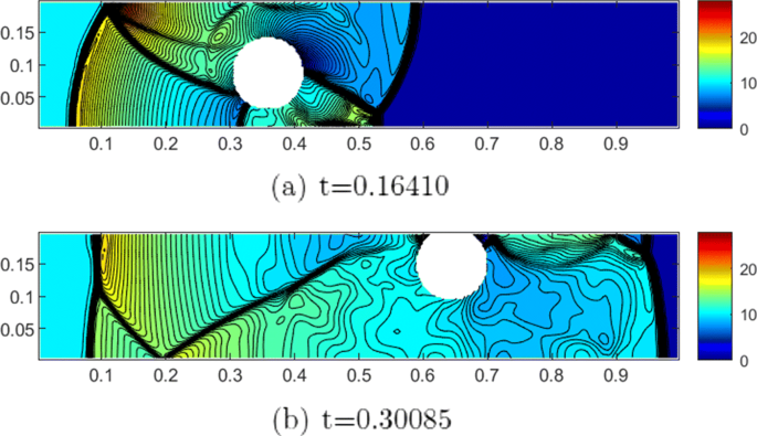

  

  The example 5.2: pressure contours of compressible inviscid fluid around a 3D cylinder. M_s=3

• Compressible viscous fluid. We take Re=1000,Pr=0.7, and $T_{b}=\frac {5}{7}$. We plot the pressure contour in Fig. 2 along the cross section of z=0 at two typical time points.

  Fig. 2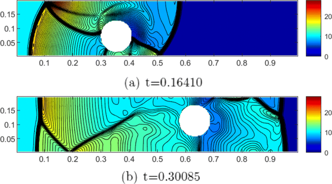

  

  The example 5.2: pressure contours of compressible viscous fluid around a 3D cylinder. M_s=3

Our numerical results consist with those of two dimensional ones in [13, 28], indicating our method for three dimensional problems is correct.

5.3 Interaction between shock wave and a sphere

The computational domain is taken as [x_l,x_r]×[y_l,y_r]×[z_l,z_r]=[0,1]×[0,0.2]×[−0.5,0.5]. The initial position of the spherical center is (0.15,0.05,0), with the radius r=0.05 and the density σ=10.77. And a shock wave is located at x=0.08 initially. We test the example with M_s=3 and M_s=6.

In the early stage of computation, the sphere is impacted by the shock wave to produce a reflected shock wave, and the reflected shock wave hits the lower wall to generate a new reflected shock wave, causing uneven pressure distribution on the upper and lower sides of the sphere. The uneven pressure causes the sphere to move upward. Figures 3 and 4 show this procedure for inviscid fluid and viscous fluid respectively.

Fig. 3

The example 5.3: the early stage of the interaction of a plane shock wave and a sphere in inviscid case for Mach number M_s=3. Pressure contours along z=0

Fig. 4

The example 5.3: the early stage of the interaction of a plane shock wave and a sphere in viscous case for Mach number M_s=3,Re=1000. Pressure contours along z=0

Later, the reflections of Mach shocks from the walls reach the sphere, generating more structures. Those structures will vary with the fluid.

• Compressible inviscid fluid. Figures 5, 6 and 7 contain the time evolution of the interaction of a plane shock wave and a sphere for Mach number M_s=3 and M_s=6 respectively. The pressure contours along the cross section of z=0 are plotted. We can observe that there is a reflected shock wave when the incident shock wave interacts with the sphere. There is a second reflected shock wave when the reflected shock wave interacts with the upper wall. The second reflected shock wave hits the sphere again and forms a secondary interaction. The rigid body would be under greater stress in fluid with a larger Mach number. Consequently, the body would move faster. These numerical results show that our numerical method is robust in the computation for the supersonic flow with high Mach number.

  Fig. 5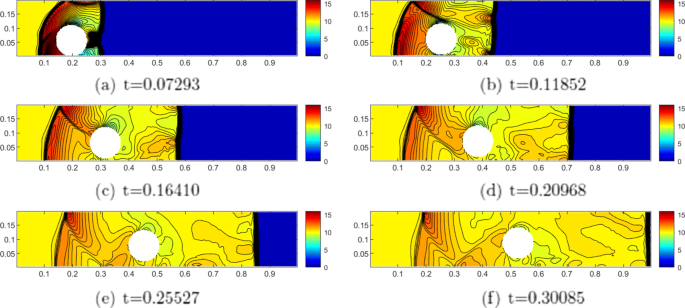

  

  The example 5.3: the time evolution of the interaction of a plane shock wave and a sphere in inviscid case for Mach number M_s=3. Pressure contours along z=0

  Fig. 6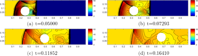

  

  The example 5.3: the time evolution of the interaction of a plane shock wave and a sphere in inviscid case for Mach number M_s=6. Pressure contours along z=0

  Fig. 7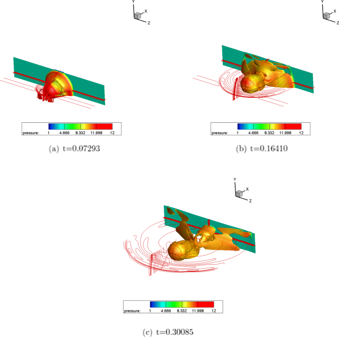

  

  The example 5.3: The iso-surface of vorticity ω=15 of the interaction of a plane shock wave and a sphere in inviscid case for Mach number M_s=3. The red line is the contour of pressure on xy- and xz-section plane going through the center of the sphere

• Compressible viscous fluid. We take Re=500 and 10⁷,Pr=0.7, and $T_{b}=\frac {5}{7}$. The time evolution of the interaction of a plane shock wave and a sphere for Mach number M_s=3 and M_s=6 is plotted in Figs. 8, 9, 10, 11 and 12. Again, the system of shock waves is observed clearly, and results are significantly different with different Mach numbers. However, there is no discernible difference when changing Reynold number.

  Fig. 8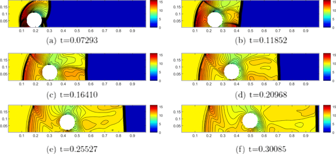

  

  The example 5.3: the time evolution of the interaction of a plane shock wave and a sphere in viscous case for Mach number M_s=3 and Re=500. Pressure contours along z=0

  Fig. 9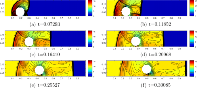

  

  The example 5.3: the time evolution of the interaction of a plane shock wave and a sphere in viscous case for Mach number M_s=3 and Re=10⁷. Pressure contours along z=0

  Fig. 10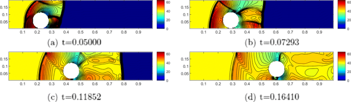

  

  The example 5.3: the time evolution of the interaction of a plane shock wave and a sphere in viscous case for Mach number M_s=6 and Re=500. Pressure contours along z=0

  Fig. 11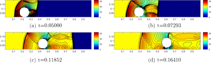

  

  The example 5.3: the time evolution of the interaction of a plane shock wave and a sphere in viscous case for Mach number M_s=6 and Re=10⁷. Pressure contours along z=0

  Fig. 12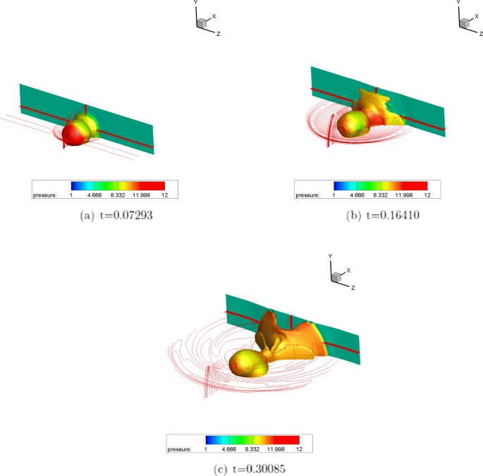

  

  The example 5.3: The iso-surface of vorticity ω=15 of the interaction of a plane shock wave and a sphere in viscous case for Mach number M_s=3 and Re=500. The red line is the contour of pressure on xy- and xz-section plane going through the center of the sphere

In addition, 3D pictures of the iso-surface of vorticity and the contour of pressure of the inviscid fluid and viscous fluid are given in Figs. 7 and 12, respectively. The numerical results demonstrate that our methods are stable and efficient for general cases.

6 Conclusion

In this paper, we develop the high order numerical boundary treatments for compressible inviscid fluid and viscous fluid, and further use them to simulate the interaction between a complex moving rigid body and a shock wave in 3D. Schemes are based on the finite difference methods on fixed Cartesian meshes in complex moving geometries. Values on the ghost points can be obtained through a Taylor expansion on the boundary in the normal direction. And we can construct point values and normal derivatives via ILW procedure or extrapolation, or their combination according to the equations and boundary conditions. This is an extension of our works [13, 28], in which the boundary treatment was designed for 2D problems. Different from the 2D case, the local coordinate rotation required in the ILW procedure is not unique in 3D. We prove that the choice of the rotation will not affect results of the boundary treatment. Hence, we can choose a simple one in our simulation. On the other hand, the material derivative for inviscid fluid on the moving boundary with no-penetration condition is newly given. Consequently, we can simulate the body with both translation and rotation. In the numerical tests, we show the results of cylinder and sphere, indicating our algorithm is effective and robust.

7 Appendix A: WENO method

Numerical fluxes $\hat {\mathbf {F}}_{i+1/2,j,k}, \hat {\mathbf {G}}_{i,j+1/2,k}$ and $\hat {\mathbf {H}}_{i,j,k+1/2}$ can be approximated in a dimension- by-dimension fashion. This means the numerical flux $\hat {\mathbf {F}}_{i+1/2,j,k}$ is obtained by the one dimensional WENO reconstruction with j and k fixed. Likewise, the numerical flux $\hat {\mathbf {G}}_{i,j+1/2,k}$ (or $\hat {\mathbf {H}}_{i,j,k+1/2}$) is obtained by one dimensional approximation procedure with i and k (or i and j) fixed. In the following part, we give the details of the third order WENO procedure to construct $\hat {\mathbf {F}}_{i+1/2,j,k}$. And for ease of notation, we ignore the indexes j and k here.

• 1. Compute an average state W_i+1/2, using either the simple arithmetic mean

  $$\mathbf{W}_{i+1/2} = \frac{1}{2} \left(\mathbf{W}_{i} + \mathbf{W}_{i+1} \right),$$

  or a Roe average satisfying

  $$\mathbf{F}' (\mathbf{W}_{i+1/2}) (\mathbf{W}_{i+1} - \mathbf{W}_{i}) = \mathbf{F}(\mathbf{W}_{i+1}) - \mathbf{F}(\mathbf{W}_{i});$$

• 2. Compute the right eigenvectors, the left eigenvectors, and the eigenvalues of the Jacobian F^′(W_i+1/2), and denote them by

  $$\mathbf{R} = \mathbf{R}(\mathbf{W}_{i+1/2}), \quad \mathbf{R}^{-1} = \mathbf{R}^{-1}(\mathbf{W}_{i+1/2}), \quad \mathbf{\Lambda} = \mathbf{\Lambda}(\mathbf{W}_{i+1/2}); $$

• 3. Transform all the point values W_j and fluxes F_j=F(W_j) which are in the potential stencil of the WENO reconstruction to the local characteristic fields:

  $$\tilde{\mathbf{W}}_{j} = \mathbf{R}^{-1} \mathbf{W}_{j}, \quad \tilde{\mathbf{F}}_{j} = \mathbf{R}^{-1} \mathbf{F}_{j}, \quad j=i-1,\ldots, i+2; $$

• 4. Do the flux splitting:

  $$\tilde{\mathbf{F}}^{\pm}_{j} = \frac{1}{2} \left(\tilde{\mathbf{F}}_{j} \pm \alpha \tilde{\mathbf{W}}_{j} \right), \quad j=i-1,\ldots,i+2, $$

  where, α= maxl|λ_l(F^′(W))| takes over the relevant range of W, and λ_l are the eigenvalues of the Jacobian F^′(W);

• 5. Perform the scalar WENO reconstruction procedure for each component of $\tilde {\mathbf {F}}^{+}=\left (\tilde {f}^{+}_{1}, \ldots, \tilde {f}^{+}_{5}\right)^{T}$ on the left-biased stencil to obtain the corresponding component of the fluxes $\hat {\tilde {\mathbf {F}}}^{+}_{i+1/2} = \left (\left (\hat {\tilde {f}}_{1}\right)^{+}_{i+1/2}, \cdots, (\hat {\tilde {f}}_{5})^{+}_{i+1/2} \right)^{T}$. We summarize the procedure for each component l=1,…,5 :

  • (a) On the two small stencils S⁽¹⁾={x_i−1,x_i} and S⁽²⁾={x_i,x_i+1}, we have the low order approximation

    $$\begin{aligned} & (\hat{\tilde{f}}_{l})^{(1)}_{i+1/2} = -\frac{1}{2} (\tilde{f}_{l})_{i-1} + \frac{3}{2} (\tilde{f}_{l})_{i}, \\ & (\hat{\tilde{f}}_{l})^{(2)}_{i+1/2} = \frac{1}{2} (\tilde{f}_{l})_{i} + \frac{1}{2} (\tilde{f}_{l})_{i+1}, \end{aligned} $$

    and the linear weights

    $$d_{1}=\frac{1}{3}, \quad d_{2}=\frac{2}{3};$$

  • (b) Change the linear weights d_r to nonlinear weights ω_r:

    $$\omega_{r} = \frac{\alpha_{r}}{\alpha_{1} +\alpha_{2}}, \quad \alpha_{r} = \frac{d_{r}}{(\beta_{r}+\epsilon)^{2},}, \quad r=1,2, $$

    with ε=10⁻⁶ to avoid the denominator being zero, and the smoothness indicators β_r on each small stencil are given as

    $$\begin{aligned} & \beta_{1} = \left((\tilde{f}_{l})_{i-1} - (\tilde{f}_{l})_{i}\right)^{2}, \\ & \beta_{2} = \left((\tilde{f}_{l})_{i} - (\tilde{f}_{l})_{i+1}\right)^{2}; \end{aligned} $$

  • (c) Find the third order reconstruction

    $$(\hat{\tilde{f}}_{l})^{+}_{i+1/2} = \omega_{1} (\hat{\tilde{f}}_{l})^{(1)}_{i+1/2} + \omega_{2} (\hat{\tilde{f}}_{l})^{(2)}_{i+1/2}; $$

• 6. Construct $\hat {\tilde {\mathbf {F}}}^{-}_{i+1/2}$ based on $\tilde {\mathbf {F}}^{-}$ and the right-biased stencil. The process to obtain $\hat {\tilde {\mathbf {F}}}^{-}_{i+1/2}$ is mirror-symmetric to that for $\hat {\tilde {\mathbf {F}}}^{+}_{i+1/2}$, with respect to the target point x_i+1/2;

• 7. Form the numerical flux as

  $$\hat{\tilde{\mathbf{F}}}_{i+1/2} = \hat{\tilde{\mathbf{F}}}^{+}_{i+1/2} + \hat{\tilde{\mathbf{F}}}^{-}_{i+1/2} ;$$

• 8. Transform back into physical space

  $$\hat{\mathbf{F}}_{i+1/2} = \mathbf{R} \, \hat{\tilde{\mathbf{F}}}_{i+1/2}.$$

8 Appendix B: A proof of Theorem 1

We prove the boundary treatment of the Euler equation here. The theorem also holds for the Navier-Stokes equation, and the proof is similar.

As before, assume P_i,j,k=(x_i,y_j,z_k) is the ghost point we are concerned about, P_a is its pedal point at the boundary, and n=(n₁,n₂,n₃) is the normal vector which points from P_a to P_i,j,k. We choose $\mathbf {t}^{1}=\left (t^{1}_{1},t^{1}_{2},t^{1}_{3}\right), \mathbf {t}^{2}=\left (t^{2}_{1},t^{2}_{2},t^{2}_{3}\right)$ as two orthogonal tangent vectors to take the rotation. The rotation matrix can be written as follows:

$$ \mathbf{T} =\left(\begin{array}{ccc} n_{1} & n_{2} & n_{3} \\ t^{1}_{1} & t^{1}_{2} & t^{1}_{3} \\ t^{2}_{1} & t^{2}_{2} & t^{2}_{3} \\ \end{array}\right). $$

With this rotation, we have:

$$\left(\begin{array}{c}\hat{u}_{a,ext}^{(k)}\\ \hat{v}_{a,ext}^{(k)}\\ \hat{w}_{a,ext}^{(k)}\end{array}\right)=\mathbf{T}\left(\begin{array}{c}u_{a,ext}^{(k)}\\ v_{a,ext}^{(k)}\\ w_{a,ext}^{(k)}\end{array}\right), \quad k=0,1,2 $$

where $u_{a,ext}^{(k)}, v_{a,ext}^{(k)}, w_{a,ext}^{(k)}$ can be obtained by extrapolation without using t¹ and t². And the local characteristic decomposition can be written as:

$${}\left(\!\begin{array}{c} (\hat{V}_{1})_{a}^{(k)}\\ (\hat{V}_{2})_{a}^{(k)}\\ (\hat{V}_{3})_{a}^{(k)}\\ (\hat{V}_{4})_{a}^{(k)}\\ (\hat{V}_{5})_{a}^{(k)}\end{array}\!\right) \,=\,\mathbf{L}_{a} \left(\!\begin{array}{c} \rho_{a,ext}^{(k)}\\ \hat{u}_{a,ext}^{(k)}\\ \hat{v}_{a,ext}^{(k)}\\ \hat{w}_{a,ext}^{(k)}\\ p_{a,ext}^{(k)}\\ \end{array}\!\right) \,=\, \left(\!\begin{array}{ccccc} 0&-\frac{1}{2}\sqrt{\gamma p_{a,ext}^{(0)} \rho_{a,ext}^{(0)}} & 0 & 0 &\frac{1}{2}\\ 0& 0 & 0 & 1 & 0\\ 0& 0 & 1 & 0 & 0\\ 1& 0 & 0 & 0 & -\frac{\rho_{a,ext}^{(0)}}{\sqrt{p_{a,ext}^{(0)}}}\\ 0&\frac{1}{2}\sqrt{\gamma p_{a,ext}^{(0)} \rho_{a,ext}^{(0)}} & 0 & 0 &\frac{1}{2}\\ \end{array}\!\right)\! \left(\!\begin{array}{c} \rho_{a,ext}^{(k)}\\ \hat{u}_{a,ext}^{(k)}\\ \hat{v}_{a,ext}^{(k)}\\ \hat{w}_{a,ext}^{(k)}\\ p_{a,ext}^{(k)}\\ \end{array}\!\right), \quad k=0,1,2 $$

Substitute the above characteristic variables into the right-hand-term of equation (27) and solve the linear system, we get:

$${}\left\{ \begin{aligned} &\left(\hat{U}_{1}\right)^{(0)}=\rho_{a,ext}^{(0)}\left(1+\sqrt{\frac{\rho_{a,ext}^{(0)}}{\gamma p_{a,ext}^{(0)}}} \left(\hat{u}_{a,ext}^{(0)}-\hat{u}_{b} \right) \right), \\ &\left(\hat{U}_{2}\right)^{(0)}=\hat{u}_{b}-\left(n_{1} u_{a,ext}^{(0)} + n_{2} v_{a,ext}^{(0)} + n_{3} w_{a,ext}^{(0)}\right)+\left(n_{1} u_{a,ext}^{(0)} + n_{2} v_{a,ext}^{(0)} + n_{3} w_{a,ext}^{(0)}\right), \\ &\left(\hat{U}_{3}\right)^{(0)}=t^{1}_{1} u_{a,ext}^{(0)} + t^{1}_{2} v_{a,ext}^{(0)} + t^{1}_{3} w_{a,ext}^{(0)}, \\ &\left(\hat{U}_{4}\right)^{(0)}=t^{2}_{1} u_{a,ext}^{(0)} + t^{2}_{2} v_{a,ext}^{(0)} + t^{2}_{3} w_{a,ext}^{(0)}, \\ &\left(\hat{U}_{5}\right)^{(0)}=p_{a,ext}^{(0)}+\sqrt{\gamma \rho_{a,ext}^{(0)} \, p_{a,ext}^{(0)}} \, \left(\hat{u}_{a,ext}^{(0)}-\hat{u}_{b} \right). \end{aligned} \right. $$

Apply the relation

$$ \mathbf{U}^{(k)} = \left(\begin{array}{ccccc} 1& 0 & 0 & 0 & 0\\ 0& n_{1} & t^{1}_{1} & t^{2}_{1} & 0\\ 0& n_{2} & t^{1}_{2} & t^{2}_{2} & 0\\ 0& n_{3} & t^{1}_{3} & t^{2}_{3} & 0\\ 0& 0 & 0 & 0 & 1\\ \end{array}\right) \hat{\mathbf{U}}^{(k)}, \quad k=0,1,2. $$

(45)

We have

$$\left\{ \begin{aligned} &(U_{1})^{(0)}=\rho_{a,ext}^{(0)}\left(1+\sqrt{\frac{\rho_{a,ext}^{(0)}}{\gamma p_{a,ext}^{(0)}}} \left(\hat{u}_{a,ext}^{(0)}-\hat{u}_{b} \right)\right), \\ &(U_{2})^{(0)}=n_{1}\left(\hat{u}_{b}-\left(n_{1} u_{a,ext}^{(0)} + n_{2} v_{a,ext}^{(0)} + n_{3} w_{a,ext}^{(0)}\right)\right) + u_{a,ext}^{(0)}, \\ &(U_{3})^{(0)}=n_{2}\left(\hat{u}_{b}-\left(n_{1} u_{a,ext}^{(0)} + n_{2} v_{a,ext}^{(0)} + n_{3} w_{a,ext}^{(0)}\right)\right) + v_{a,ext}^{(0)}, \\ &(U_{4})^{(0)}=n_{3}\left(\hat{u}_{b}-\left(n_{1} u_{a,ext}^{(0)} + n_{2} v_{a,ext}^{(0)} + n_{3} w_{a,ext}^{(0)}\right)\right) + w_{a,ext}^{(0)}, \\ &(U_{5})^{(0)}=p_{a,ext}^{(0)}+\sqrt{\gamma \rho_{a,ext}^{(0)} \, p_{a,ext}^{(0)}} \left(\hat{u}_{a,ext}^{(0)}-\hat{u}_{b} \right). \end{aligned} \right. $$

Here, the orthogonality of rotation matrix T is used. And we can see that all the terms here are independent of t¹ and t².

Similarly, substitute the characteristic variables into equation (28) and solve the linear system, we get:

$$\left\{ \begin{aligned} &(\hat{U}_{1})^{(1)}=\rho_{a,ext}^{(1)}+\rho_{a,ext}^{(0)}\left(\frac{\rho_{a,ext}^{(0)}\frac{D\hat{u}}{Dt}-p_{a,ext}^{(1)}}{\gamma p_{a,ext}^{(0)}}+\frac{D\hat{u}}{Dt}\left(\frac{\rho_{a,ext}^{(0)}}{\gamma p_{a,ext}^{(0)}}\right)^{\frac{3}{2}}\left(\hat{u}_{a,ext}^{(0)}-\hat{u}_{b}\right)\right), \\ &(\hat{U}_{2})^{(1)}=n_{1} u_{a,ext}^{(1)} + n_{2} v_{a,ext}^{(1)} + n_{3} w_{a,ext}^{(1)}+\hat{u}_{res}, \\ &(\hat{U}_{3})^{(1)}=t^{1}_{1} u_{a,ext}^{(1)} + t^{1}_{2} v_{a,ext}^{(1)} + t^{1}_{3} w_{a,ext}^{(1)}, \\ &(\hat{U}_{4})^{(1)}=t^{2}_{1} u_{a,ext}^{(1)} + t^{2}_{2} v_{a,ext}^{(1)} + t^{2}_{3} w_{a,ext}^{(1)}, \\ &(\hat{U}_{5})^{(1)}=\rho_{a,ext}^{(0)}\frac{D\hat{u}}{Dt} \left(1+\sqrt{\frac{\rho_{a,ext}^{(0)}}{\gamma p_{a,ext}^{(0)}}}\left(\hat{u}_{a,ext}^{(0)}-\hat{u}_{b}\right)\right), \end{aligned} \right. $$

where

$$\frac{D\hat{u}}{Dt}=\hat{\mathbf{u}}\cdot\frac{D\hat{\mathbf{n}}}{Dt}-\frac{d}{dt}(\mathbf{V}_{b}\cdot\mathbf{n}) $$

and

$$\hat{u}_{res}=-\frac{\rho_{a,ext}^{(0)}\frac{D\hat{u}}{Dt}-p_{a,ext}^{(1)}}{\sqrt{\gamma p_{a,ext}^{(0)} \rho_{a,ext}^{(0)}}}+\frac{D\hat{u}}{Dt}\frac{\rho_{a,ext}^{(0)}}{\gamma p_{a,ext}^{(0)}}\left(\hat{u}_{a,ext}^{(0)}-\hat{u}_{b}\right)$$

are terms which are independent of t¹ and t².

Apply the relation (45), we get

$$\left\{ \begin{aligned} &(U_{1})^{(1)}=\rho_{a,ext}^{(1)}+\rho_{a,ext}^{(0)}\left(\frac{\rho_{a,ext}^{(0)}\frac{D\hat{u}}{Dt}-p_{a,ext}^{(1)}}{\gamma p_{a,ext}^{(0)}}+\frac{D\hat{u}}{Dt} \left(\frac{\rho_{a,ext}^{(0)}}{\gamma p_{a,ext}^{(0)}}\right)^{\frac{3}{2}} \left(\hat{u}_{a,ext}^{(0)}-\hat{u}_{b}\right)\right), \\ &(U_{2})^{(1)}=n_{1} \hat{u}_{res} + u_{a,ext}^{(1)}, \\ &(U_{3})^{(1)}=n_{2} \hat{u}_{res} + v_{a,ext}^{(1)}, \\ &(U_{4})^{(1)}=n_{3} \hat{u}_{res} + w_{a,ext}^{(1)}, \\ &(U_{5})^{(1)}=\rho_{a,ext}^{(0)}\frac{D\hat{u}}{Dt} \left(1+\sqrt{\frac{\rho_{a,ext}^{(0)}}{\gamma p_{a,ext}^{(0)}}}\left(\hat{u}_{a,ext}^{(0)}-\hat{u}_{b}\right)\right). \end{aligned} \right. $$

Again, we can see the expression of $\mathbf {U}_{a}^{(1)}$ does not explicitly contain t¹ and t². Also, the second order derivative $\mathbf {U}_{a}^{(2)}$, which is obtained by extrapolation directly, can be got without using the tangent vectors.

Therefore, the ghost points can be defined by a Taylor expansion without tangent vectors.

9 Appendix C: WENO extrapolation

The idea of WENO extrapolation is using nonlinear weights to combine the approximations on candidate substencils.

Firstly, we select three candidate substencils S₀,S₁,S₂ for extrapolation. There is more than one way to select them. Thanks to the regular boundaries like a sphere, we can simplify the traditional point finding method in [17]. Here, the inner lattice points whose distance from point P_a is less than 1.1h,2.1h and 3.1h are grouped to compose S₀,S₁,S₂ respectively, where h= max(Δx,Δy,Δz) is the largest mesh size.

Then, for each component of V, we reconstruct a polynomial of p_m(x,y,z) (m=0,1,2) with the least square method on each candidate substencil S_m, respectively. Values of $\frac {\partial ^{k} V_{i}}{\partial \hat {x}^{k}}$(i=1,2,3,4) can be extrapolated as:

$$ \frac{\partial^{k} V_{i}}{\partial \hat{x}^{k}}=\sum_{m=0}^{2}d_{m}\frac{\partial^{k}}{\partial \hat{x}^{k}}p_{m}|_{(x,y,z)=(x_{(a)},y_{(a)},z_{(a)})} $$

(46)

where $d_{0}=\Delta x^{2}+\Delta y^{2}+\Delta z^{2}, d_{1}=\sqrt {\Delta x^{2}+\Delta y^{2}+\Delta z^{2}}, d_{2}=1-d_{0}-d_{1}$.

Next, we change the approximation (46) to a WENO type extrapolation to avoid spurious oscillation, with the following form:

$$ \frac{\partial^{k} V_{i}}{\partial \hat{x}^{k}}=\sum_{m=0}^{2}\omega_{m}\frac{\partial^{k}}{\partial \hat{x}^{k}}p_{m}|_{(x,y,z)=(x_{(a)},y_{(a)},z_{(a)})}, $$

(47)

where ω₀,ω₁,ω₂ are nonlinear weights depending on the smoothness of the functions on candidate substencils, taken as

$$ \omega_{m}=\frac{\alpha_{m}}{\sum_{s=0}^{2}\alpha_{s}}, \quad m=0,1,2, $$

(48)

with

$$ \alpha_{m}=\frac{d_{m}}{(\epsilon+\beta_{m})^{2}}. $$

(49)

The small number ε is taken as 10⁻⁶ to avoid zero denominator. The smoothness indicators β_m are similar to those in [31]

$$ \begin{aligned} \beta_{0}&=\Delta x^{2}+\Delta y^{2}+\Delta z^{2}, \\ \beta_{m}&=\sum_{1\le|\mu|\le m}\iiint_{K} |K|^{2/3|\mu|-1}(D^{\mu} p_{m})^{2}dxdydz \end{aligned} $$

(50)

where μ is a muti-index and K =[x_(a)−Δx/2,x_(a)+Δx/2]×[y_(a)−Δy/2,y_(a)+Δy/2]×[z_(a)−Δz/2,z_(a)+Δz/2]. With the careful design of nonlinear weights ω_m, the WENO extrapolation can meet third order accuracy when the function is smooth enough on all candidate substencils.

References

Berger MJ, Helzel C, Leveque RJ (2003) h-box methods for the approximation of hyperbolic conservation laws on irregular grids. SIAM J Numer Anal 41:893–918.
Baeza A, Mulet P, Zoro D (2016) High order accurate extrapolation technique for finite difference methods on complex domains with Cartesian meshes. J Sci Comput 66:761–791.
Kreiss H-O, Petersson NA (2006) A second order accurate embedded boundary method for the wave equation with Dirichlet data. SIAM J Sci Comput 27:1141–1167.
Kreiss H-O, Petersson NA, Yström J (2002) Difference approximations for the second order wave equation. SIAM J Numer Anal 40:1940–1967.
Kreiss H-O, Petersson NA, Yström J (2004) Difference approximations of the Neumann problem for the second order wave equation. SIAM J Numer Anal 42:1292–1323.
Nilsson S, Petersson NA, Sjögreen B, Kreiss H-O (2007) Stable difference approximations for the elastic wave equation in second order formulation. SIAM J Numer Anal 45:1902–1936.
Sjögreen B, Petersson NA (2007) A Cartesian embedded boundary method for hyperbolic conservation laws. Commun Comput Phys 2:1199–1219.
Mittal R, Iaccarino G (2005) Immersed boundary methods. Ann Rev Fluid Mech 37:239–261.
Peskin CS (2002) The immersed boundary method. Acta Numerica 11:1–39.
Qu Y, Shi R, Batra RC (2018) An immersed boundary formulation for simulating high-speed compressible viscous flows with moving solids. J Comput Phys 354:672–691.
Vanna FD, Picano F, Benini E (2020) A sharp-interface immersed boundary method for moving objects in compressible viscous flows. Comput Fluids 201:104415.
Wang J, Gu X, Wu J (2020) A sharp-interface immersed boundary method for simulating high-speed compressible inviscid flows. Adv Appl Math Mech 12:545–563.
Cheng Z, Liu S, Jiang Y, Lu J, Zhang M, Zhang S (2021) A high order boundary scheme to simulate a complex moving rigid body under the impingement of a shock wave. Appl Math Mech (Engl Ed) 42:841–854.
Ding S, Shu C-W, Zhang M (2020) On the conservation of finite difference WENO schemes in non-rectangular domains using the inverse Lax-Wendroff boundary treatments. J Comput Phys 415:109516.
Lu J, Fang J, Tan S, Shu C-W, Zhang M (2016) Inverse Lax-Wendroff procedure for numerical boundary conditions of convection-diffusion equations. J Comput Phys 317:276–300.
Lu J, Shu C-W, Tan S, Zhang M (2021) An inverse Lax-Wendroff procedure for hyperbolic conservation laws with changing wind direction on the boundary. J Comput Phys 426:109940.
Tan S, Shu C-W (2010) Inverse Lax-Wendroff procedure for numerical boundary conditions of conservation laws. J Comput Phys 229:8144–8166.
Tan S, Shu C-W (2011) A high order moving boundary treatment for compressible inviscid flows. J Comput Phys 230:6023–6036.
Tan S, Shu C-W (2013) Inverse Lax-Wendroff procedure for numerical boundary conditions of hyperbolic equations: survey and new developments. In: Melnik R Kotsireas I (eds)Advances in Applied Mathematics, Modeling and Computational Science, 41–63.. Fields Institute Communications 66, Springer, New York.
Tan S, Wang C, Shu C-W, Ning J (2012) Efficient implementation of high order inverse Lax-Wendroff boundary treatment for conservation laws. J Comput Phys 231:2510–2527.
Huang L, Shu C-W, Zhang M (2008) Numerical boundary conditions for the fast sweeping high order WENO methods for solving the Eikonal equation. J Comput Math 26:336–346.
Xiong T, Zhang M, Zhang Y-T, Shu C-W (2010) Fifth order fast sweeping WENO scheme for static Hamilton-Jacobi equations with accurate boundary treatment. J Sci Comput 45:514–536.
Filbet F, Yang C (2013) An inverse Lax–Wendroff method for boundary conditions applied to Boltzmann type models. J Comput Phys 245:43–61.
Li T, Shu C-W, Zhang M (2017) Stability analysis of the inverse Lax-Wendroff boundary treatment for high order central difference schemes for diffusion equations. J Sci Comput 70:576–607.
Li T, Lu J, Shu C-W (2021) Stability analysis of inverse Lax-Wendroff boundary treatment of high order compact difference schemes for parabolic equations. J Comput Appl Math 400:113711.
Li T, Shu C-W, Zhang M (2016) Stability analysis of the inverse Lax-Wendroff boundary treatment for high order upwind-biased finite difference schemes. J Comput Appl Math 299:140–158.
Vilar F, Shu C-W (2015) Development and stability analysis of the inverse Lax-Wendroff boundary treatment for central compact schemes. ESAIM Math Model Numer Anal (M2AN) 49:39–67.
Liu S, Jiang Y, Shu C-W, Zhang M, Zhang S (2021) A high order moving boundary treatment for convection-diffusion equations. https://www.brown.edu/research/projects/scientific-computing/sites/brown.edu.research.projects.scientific-computing/files/uploads/A%20high%20order%20moving%20boundary%20treatment.pdf.
Jiang G-S, Shu C-W (1996) Efficient implementation of weighted ENO schemes. J Comput Phys 126:202–228.
Shu C-W, Osher S (1988) Efficient implementation of essentially non-oscillatory shock-capturing schemes. J Comput Phys 77:439–471.
Zhang Y-T, Shu C-W (2009) Third order WENO scheme on three dimensional tetrahedral meshes. Commun Comput Phys 5:836–848.
Acknowledgments
N/A.
Funding
This work has been supported by the National Numerical Windtunnel project (No. NNW2019ZT4-B10), and the National Natural Science Foundation of China (Nos. 11901555, 11901213, 11871448, 11732016).
Author information
Authors and Affiliations
Contributions
All the authors contributed to and approved this manuscript.
Corresponding author
Ethics declarations
Competing interests
The authors declare that they have no competing interests.
Additional information
Publisher’s Note
Springer Nature remains neutral with regard to jurisdictional claims in published maps and institutional affiliations.
Rights and permissions
Open Access This article is licensed under a Creative Commons Attribution 4.0 International License, which permits use, sharing, adaptation, distribution and reproduction in any medium or format, as long as you give appropriate credit to the original author(s) and the source, provide a link to the Creative Commons licence, and indicate if changes were made. The images or other third party material in this article are included in the article’s Creative Commons licence, unless indicated otherwise in a credit line to the material. If material is not included in the article’s Creative Commons licence and your intended use is not permitted by statutory regulation or exceeds the permitted use, you will need to obtain permission directly from the copyright holder. To view a copy of this licence, visit http://creativecommons.org/licenses/by/4.0/.
About this article
Cite this article
Liu, S., Cheng, Z., Jiang, Y. et al. Numerical simulation of a complex moving rigid body under the impingement of a shock wave in 3D. Adv. Aerodyn. 4, 8 (2022). https://doi.org/10.1186/s42774-021-00096-5
Received:
Accepted:
Published:
DOI: https://doi.org/10.1186/s42774-021-00096-5