Adaptive local discontinuous Galerkin methods with semi-implicit time discretizations for the Navier-Stokes equations

Abstract

In this paper, we present a mesh adaptation algorithm for the unsteady compressible Navier-Stokes equations under the framework of local discontinuous Galerkin methods coupled with implicit-explicit Runge-Kutta or spectral deferred correction time discretization methods. In both of the two high order semi-implicit time integration methods, the convective flux is treated explicitly and the viscous and heat fluxes are treated implicitly. The remarkable benefits of such semi-implicit temporal discretizations are that they can not only overcome the stringent time step restriction compared with time explicit methods, but also avoid the construction of the large Jacobian matrix as is done for fully implicit methods, thus are relatively easy to implement. To save computing time as well as capture the flow structures of interest accurately, a local mesh refinement (h-adaptive) technique, in which we present detailed criteria for selecting candidate elements and complete strategies to refine and coarsen them, is also applied for the Navier-Stokes equations. Numerical experiments are provided to illustrate the high order accuracy, efficiency and capabilities of the semi-implicit schemes in combination with adaptive local discontinuous Galerkin methods for the Navier-Stokes equations.

1 Introduction

In this paper, we focus on an h-adaptive local discontinuous Galerkin (LDG) method in combination with implicit-explicit Runge-Kutta (IMEX-RK) or spectral deferred correction (SDC) time discretizations to solve the unsteady compressible Navier-Stokes (NS) equations.

The discontinuous Galerkin (DG) method, which is a class of finite element methods using a completely discontinuous piecewise polynomial space for the numerical solutions and the test functions in spatial variables, has been widely used in computational fluid dynamics, computational acoustics and computational magneto-hydrodynamics, since it was firstly introduced in 1973 by Reed and Hill [1] in the framework of linear neutron transport and then further extended by Cockburn et al. [2–5] for solving nonlinear hyperbolic conservation laws through a combination of explicit, Strong-Stability-Preserving Runge-Kutta (SSP-RK) time discretizations and total variation bounded nonlinear limiters to achieve non-oscillatory properties for strong shocks. The DG methods combine two advantageous features commonly associated to continuous finite element and finite volume methods, such as high order accuracy, flexibility on complex geometry, flexibility for h-p adaptivity, and so on, and are indeed a natural consideration when solving hyperbolic conservation laws, such as the compressible Euler equations. However, when it comes to partial differential equations (PDEs) containing high order spatial derivatives, e.g., the compressible NS equations where the viscous and heat fluxes exist, a severe difficulty with the approximations of the numerical fluxes for solution derivatives arises by the direct application of the DG methods, and a naive arithmetic mean of the solution derivatives without taking into account the possible jump of the solutions will yield a weakly unstable scheme.

In order to properly resolve the solution derivatives in the NS equations at the interfaces, plenty of numerical methods have been proposed in the literature. In 1997, Bassi and Rebay [6] firstly attempted to apply the DG methods to the compressible NS equations, later on, they introduced an improved method [7] based on the previous scheme in order to maintain the compactness and stability for the pure diffusion problems. Hartmann and Houston [8] proposed employing the symmetric interior penalty method, which can guarantee optimal order of convergence in terms of L² norm of the error, for the discretization of the leading order terms of the compressible NS equations. To deal with moving and deforming boundaries, Klaij and van der Vegt [9] presented a space-time DG method for the compressible NS equations. The key feature of the space-time DG method is that no distinction is made between space and time variables and thus this provides optimal flexibility to deal with time dependent boundaries and deforming elements. Based on a so-called inter-cell reconstruction, Luo et al. [10] developed a reconstruction-based DG method for the NS equations on arbitrary grids. The numerical viscous and heat fluxes at interfaces are obtained by locally reconstructing a smooth solution with a least-square method from the underlying discontinuous solution. Based on a direct weak formulation for the parabolic equations, a so-called direct DG method for solving second-order diffusion problems was originally introduced by Liu and Yan [11], and further extended by Cheng et al. [12] to solve the compressible NS equations.

Inspired and attracted by the high order accuracy, easy extension to high order PDEs and arbitrary grids of the LDG method, we select it as the spatial discretization in our study. Besides, adopting h-adaptive technique and semi-implicit time marching methods are another two aspects we focus on in this paper to improve the computational accuracy and efficiency as well as deduce the computational complexity. The LDG method was initially developed to solve nonlinear convection-diffusion equations by Cockburn and Shu [13], enlightened by Bassi and Rebay’s successful simulation for the compressible NS equations. The idea behind the LDG method is to properly rewrite the PDEs containing high order derivatives as a first-order system by introducing auxiliary variables, then apply the DG method to the system, in which correctly designing the numerical fluxes is the key ingredient to guarantee stability and local solvability of the auxiliary variables. There has been abundant literature on designing and analyzing the LDG schemes for different types of high order PDEs, for a detailed review, see [14] and the references therein.

By sharing the advantages of the DG method, the LDG scheme requires no imposition of solution continuity between adjacent elements and allows the appearance of hanging nodes, thus is extremely flexible to do local grid refinement. To start the mesh adaptation, a criterion to determine whether an element in the computational mesh needs to be refined or coarsened is demanded. Generally, the criteria can be divided into two types, i.e., error estimators and heuristic indicators [15]. Error estimators are based on a so-called a posteriori error estimation which seeks to bound the error with respect to a given norm. As a comparison, heuristic indicators usually depend on the local gradient of thermodynamical variables such as the density, pressure, entropy and so on, or the local divergence or curl of the velocity field, thus are relatively simple to be implemented for complicated PDEs. In the current, a rigorous mathematical analysis to develop the a posteriori error estimation for the LDG scheme of the compressible NS equations is out of our scope, therefore we consult the criteria in [16, 17] for the compressible Euler equations and choose a combination of different heuristic indicators. In practical implementation, the candidate elements marked for refinement are indeed to be refined, however, to retain the mesh quality, some other elements around these elements may also require to be refined. In contrast, to achieve the same goal, the candidate elements marked for coarsening may not be coarsened depending on their neighbors. What’s more, to maintain conservation and accuracy of the numerical solutions during refinement and coarsening, the L² projection is implemented for the prolongation and restriction of grid.

The application of any above extension of the DG methods to the compressible NS equations will generate a large coupled system of ordinary differential equations (ODEs), which require accurate and efficient time integration methods to march in time. The explicit, high order SSP-RK time discretizations, which are suitable choices for hyperbolic conservation laws, will sustain extremely small time step restriction for stability, but not for accuracy due to the appearance of stiffness terms of the NS equations, i.e., the viscous and heat fluxes terms. Nearly all the papers referred above applied the implicit temporal discretizations, e.g., the backward Euler method, to overcome this restriction. This kind of remedy is efficient to some extent, since the Courant-Friedrichs-Lewy (CFL) number can be adjusted to be quite large, but the construction of the large Jacobian matrix and the choice of efficient preconditioners for the linear systems arising in the inner loop greatly increase the difficulty in implementation. In addition, for unsteady flow problems with complicated flow structures, a time step of at least the same order of magnitude as the mesh size is required to capture the complex flow structures accurately at any time. By turning to the semi-implicit time discretization methods, specifically, IMEX-RK and SDC methods, and treating the convective, viscous and heat fluxes differently, no Jacobian matrix is required to be assembled and only two linear systems for the momentum and energy equations, respectively, need to be solved. Numerical experiments show that the residual of the GMRES solver even without any preconditioner can approach the machine error within a dozen of, sometimes two or three, outer iterations if the mesh quality is not too bad. L. Pareschi and G. Russo considered IMEX-RK methods in time for hyperbolic systems of conservation laws with stiff relaxation terms in [18]. In [19, 20] Wang et al. analyzed the stability and error estimates of the LDG methods coupled with IMEX-RK time discretizations for the linear convection-diffusion equations in one and two dimensions, and unconditional stability and optimal error estimates are obtained. Xia et al. [21] explored three different time discretization techniques including SDC methods for solving the stiff ODEs resulting from an LDG spatial discretization to PDEs containing high order spatial derivatives, and verified that all the three methods are efficient and a time step △t=O(△x) is allowed for k-th order PDEs. The LDG method is more flexible for treating the nonlinear terms when introducing the auxiliary for high order derivative terms. Due to the local properties of the LDG methods, the resulting implicit scheme is easy to implement and can be solved in an explicit way when it is coupled with iterative methods, which has been demonstrated in the references [22, 23]. For other work on semi-implicit schemes for gasdynamics, we suggest the readers consulting [24–30] and the references therein.

The outline of this paper is organized as follows. Governing equations are given in Section 2. In Section 3, we present the LDG scheme for the compressible NS equations, including the detailed and clear treatment for the numerical fluxes for subsonic inflow/outflow, supersonic inflow/outflow and solid wall boundary conditions. Section 4 is devoted to the discussion about two kinds of semi-implicit time discretization methods we adopt in this paper, i.e., IMEX-RK and SDC methods, and the fully discrete schemes of the NS equations. In Section 5 we provide the implementation details of the h-adaptive technique. Section 6 contains numerical results for the unsteady compressible NS equations, which demonstrate the high order accuracy and capabilities of the presented methods. Finally we give conclusions in Section 7.

2 Governing equations

Let $\Omega \subset \mathbb {R}^{d}$ be a bounded domain with d≤3, the NS equations governing the dynamics of viscous compressible flows express the conservation of mass, momentum and energy, and can be written in dimensionless and conservative form [31]

$$ \frac{\partial \mathbf{U}}{\partial t} + \nabla \cdot \mathbf{F}(\mathbf{U}) = \nabla \cdot \mathbf{G}(\mathbf{U}, \nabla \mathbf{U}), $$

(1)

in Ω×(0,T],T>0, with $\mathbf {U} \in \mathbb {R}^{d + 2}$ the vector of conserved variables and $\mathbf {F}, \mathbf {G} \in \mathbb {R}^{(d + 2) \times d}$ the inviscid and viscous fluxes, which are defined as

$$ \mathbf{U} = \left[\begin{array}{c} \rho \\ \rho \mathbf{u} \\ E \end{array}\right], \quad \mathbf{F} = \left[\begin{array}{c} \rho \mathbf{u} \\ \rho \mathbf{u} \otimes \mathbf{u} + p \mathbf{I} \\ (E + p) \mathbf{u} \end{array}\right], \quad \mathbf{G} = \left[\begin{array}{c} \mathbf{0} \\ \boldsymbol{\tau} \\ \boldsymbol{\tau} \mathbf{u} - \mathbf{q} \end{array}\right], $$

respectively. Here $\rho, \mathbf {u} \in \mathbb {R}^{d}$ and p denote the mass density, velocity field and pressure, respectively. I represents unit tensor. The total energy per unit volume E is the sum of internal and kinetic energy

$$ E = \rho \left(e + \frac{1}{2}|\mathbf{u}|^{2}\right), $$

with e the specific internal energy. In order to close the system, we consider the equation of state for a calorically perfect gas

$$ p = (\gamma - 1)\rho e, $$

where $\gamma = \frac {c_{p}}{c_{v}}$ is the ratio of c_p and c_v, the specific heats at constant pressure and volume, respectively. By Newtonian approximation and Stokes hypothesis, the viscous stress tensor $\boldsymbol {\tau } \in \mathbb {R}^{d \times d}$ relating to the derivatives of the velocity field u is defined as

$$ \boldsymbol{\tau} = \mu\left(\nabla \mathbf{u} + \nabla^{T} \mathbf{u} - \frac{2}{3} (\nabla \cdot \mathbf{u}) \mathbf{I}\right), $$

where the dynamic viscosity coefficient μ, which is determined through Sutherland’s law, reads in dimensionless form

$$ \mu = \frac{1}{Re_{\infty}}\frac{1 + T_{s} / T_{\infty} }{T + T_{s} / T_{\infty} }T^{\frac{3}{2}}, $$

with Re_∞ the Reynolds number, T the temperature, T_s a constant and subscript ∞ denoting the uniform free-stream values. The heat flux vector $\mathbf {q} \in \mathbb {R}^{d}$ caused by the gradient of temperature T is defined as

$$ \mathbf{q} = -\kappa \nabla T, $$

via Fourier’s heat conduction law, where $\kappa = \frac {c_{p} \mu }{Pr}$ is the thermal conductivity coefficient, with Pr the Prandtl number. In addition, the specific internal energy e can relate to the temperature T by

$$ e = c_{v} T. $$

As a matter of fact, the specific heats c_p and c_v in dimensionless form can be defined as

$$ c_{p} = \frac{1}{(\gamma - 1)M_{\infty}^{2}}, \quad c_{v} = \frac{1}{\gamma(\gamma - 1)M_{\infty}^{2}}, $$

with Mach number M_∞ for uniform flow given by

$$ M_{\infty} = \frac{u_{\infty}}{a_{\infty}}, \quad a_{\infty} = \sqrt{\frac{\gamma p_{\infty}}{\rho_{\infty}}}. $$

In this paper, unless otherwise stated, we will use γ=1.4,Pr=0.72 for air, and μ as a constant for simplicity, i.e., $\mu = \frac {1}{Re_{\infty }}$.

3 The LDG method

In this section, we will introduce the LDG method for the spatial discretization of the compressible NS equations. Special attention will be paid to the numerical fluxes on various boundaries.

3.1 Notations and finite element spaces

For the DG spatial discretizations, the domain Ω is approximated with a tessellation $\mathcal {T}_{h}$ consisting of nonoverlapping shape-regular elements K, which satisfy the condition $\bigcup _{K \in \mathcal {T}_{h}} \overline {K} := \overline {\Omega }_{h} \rightarrow \overline {\Omega }$ as h→0, with the mesh size $h := \max _{K \in \mathcal {T}_{h}} h_{K}$ and the diameter h_K of element K. Let Γ denote the union of the boundaries of all the elements K and classify them into internal faces Γ_I and boundary faces Γ_B, i.e., Γ=Γ_I∪Γ_B. We also assume that Γ_B may be decomposed as follows

$$ \Gamma_{B} = \Gamma_{\mathrm{sub-in}} \cup \Gamma_{\mathrm{sub-out}} \cup \Gamma_{\mathrm{sup-in}} \cup \Gamma_{\mathrm{sup-out}} \cup \Gamma_{W}, $$

where Γ_sub−in,Γ_sub−out,Γ_sup−in,Γ_sup−out and Γ_W are distinct subsets of Γ_B representing subsonic-inflow, subsonic-outflow, supersonic-inflow, supersonic-outflow and solid wall boundaries, respectively. For solid wall boundaries, we also distinguish them either according to slip (reflective) and no-slip conditions, i.e.,

$$ \Gamma_{W} = \Gamma_{W, \text{slip}} \cup \Gamma_{W, \mathrm{no-slip}}, $$

or according to isothermal and adiabatic conditions, i.e.,

$$ \Gamma_{W} = \Gamma_{W, \text{iso}} \cup \Gamma_{W, \text{adia}}. $$

Let e∈Γ_I be an internal face shared by the “left” and “right” elements K_L and K_R, i.e., e=∂K_L∩∂K_R, where the so-called “left” and “right” can be uniquely defined for each internal face according to any fixed rule. Suppose ϕ is a function on K_L and K_R, but possibly discontinuous across e, let ϕ^L and ϕ^R denote $(\phi |_{K_{L}})|_{e}$ and $(\phi |_{K_{R}})|_{e}$, the left and right traces, respectively. Similar definitions can be obtained component-wisely for vector-valued and matrix-valued functions.

For the LDG discretizations, we require to introduce the finite element spaces. Actually each element K of the tessellation $\mathcal {T}_{h}$ is connected to a reference element $\hat {K}$ through some mapping F_K. The mapping $F_{K} : \hat {K} \rightarrow K$ from the reference element $\hat {K}$ to the real physical element K is a function defined in the space of the reference element for each independent variable. For example, for a quadrilateral element K in two dimension, $\hat {K} = [-1, 1]^{2}$ is the unit square and F_K is expressed in terms of the nodal shape functions N_i,i=1,⋯,4 by

$$ \mathbf{x} = F_{K}(\boldsymbol{\xi}) = \sum_{i = 1}^{4}\mathbf{x}_{K}^{i} N_{i}(\boldsymbol{\xi}), $$

where $\mathbf {x} = (x_{1}, x_{2}) \in K, \boldsymbol {\xi } = (\xi _{1}, \xi _{2}) \in \hat {K}, \mathbf {x}_{K}^{i}, i = 1, \cdots, 4$ are the four vertex coordinates of K and

$$\begin{array}{*{20}l} &N_{1}(\boldsymbol{\xi}) := \frac{1}{4}(1 - \xi_{1})(1 - \xi_{2}), \quad N_{2}(\boldsymbol{\xi}) := \frac{1}{4}(1 + \xi_{1})(1 - \xi_{2}), \\ &N_{3}(\boldsymbol{\xi}) := \frac{1}{4}(1 + \xi_{1})(1 + \xi_{2}), \quad N_{4}(\boldsymbol{\xi}) := \frac{1}{4}(1 - \xi_{1})(1 + \xi_{2}), \end{array} $$

see schematic map in Fig. 1. Then the finite element spaces associated with the tessellation $\mathcal {T}_{h}$ are given by

$$\begin{aligned} V_{h} &= \left\{\mathbf{V} = (v_{1}, \cdots, v_{d + 2})^{T} \in (L^{2}(\Omega))^{d + 2}: v_{i}|_{K} \circ F_{K} \in P^{k}(\hat{K}), \ i = 1, \cdots, d + 2, \ \forall K \in \mathcal{T}_{h} \right\}, \\ W_{h} &= \left\{\mathbf{W} = (w_{1}, \cdots, w_{d})^{T} \in (L^{2}(\Omega))^{d}: w_{i}|_{K} \circ F_{K} \in P^{k}(\hat{K}), \ i = 1, \cdots, d, \ \forall K \in \mathcal{T}_{h} \right\}, \\ \Sigma_{h} &= \left\{\boldsymbol{\sigma} = (\sigma_{ij})_{1 \leq i, j \leq d} \in (L^{2}(\Omega))^{d \times d}: \sigma_{ij}|_{K} \circ F_{K} \in P^{k}(\hat{K}), \ i, j = 1, \cdots, d, \ \forall K \in \mathcal{T}_{h} \right\}, \end{aligned} $$

with $P^{k}(\hat {K})$ the space of polynomials of degree up to k with respect to d variables in the reference element $\hat {K}$. Note that the functions in V_h,W_h and Σ_h are allowed to be completely discontinuous across element interfaces.

Fig. 1

Schematic map for the transformation F_K from a unit square in the reference space to the real element in the physical space

Further, we also define the inner product notations in element and on face as

$$ (\phi, \varphi)_{K} := \int_{K} \phi \varphi dK, \quad (\phi, \varphi)_{\partial{K}} := \int_{\partial{K}} \phi \varphi ds, $$

$$ (\mathbf{u}, \mathbf{v})_{K} := \int_{K} \mathbf{u} \cdot \mathbf{v} dK, \quad (\mathbf{u}, \mathbf{v})_{\partial{K}} := \int_{\partial{K}} \mathbf{u} \cdot \mathbf{v} ds, $$

$$ (\boldsymbol{\sigma}, \boldsymbol{\eta})_{K} := \int_{K} \boldsymbol{\sigma} : \boldsymbol{\eta} dK, \quad (\boldsymbol{\sigma}, \boldsymbol{\eta})_{\partial{K}} := \int_{\partial{K}} \boldsymbol{\sigma} : \boldsymbol{\eta} ds, $$

for the scalar-valued functions ϕ,φ, vector-valued functions u,v and matrix-valued functions σ,η, respectively, where

$$ \boldsymbol{\sigma} : \boldsymbol{\eta} := \sigma_{ij} \eta_{i, j}. $$

3.2 The LDG discretization

In order to propose the LDG discretization for the NS equations, we firstly rewrite (1) as a first order system, which is composed of the primary equations

$$ \frac{\partial \mathbf{U}}{\partial t} + \nabla \cdot (\mathbf{F}(\mathbf{U}) - \mathbf{G}(\mathbf{U}, \boldsymbol{\tau}, \mathbf{q})) = 0, $$

(2)

and the auxiliary equations

$$\begin{array}{*{20}l} &\mathbf{z} = \nabla \mathbf{u}, \end{array} $$

(3a)

$$\begin{array}{*{20}l} &\mathbf{q} = -\kappa \nabla T, \end{array} $$

(3b)

where U=(ρ,m,E)^T and

$$\begin{array}{*{20}l} &\mathbf{u} = \frac{\mathbf{m}}{\rho}, \end{array} $$

(4a)

$$\begin{array}{*{20}l} &\boldsymbol{\tau} = \frac{1}{Re_{\infty}} \left(\mathbf{z} + \mathbf{z}^{T} - \frac{2}{3} tr(\mathbf{z}) \mathbf{I} \right), \end{array} $$

(4b)

$$\begin{array}{*{20}l} &\kappa T = \frac{\gamma}{Re_{\infty} Pr}\left(\frac{E}{\rho} - \frac{1}{2}|\mathbf{u}|^{2}\right), \end{array} $$

(4c)

with tr(z):=z_ii the trace of the matrix z. Based on the weak formulation of (2) − (3), which is obtained by multiplying (2) −(3) by test functions, integrating over some domain, and then performing an integration by parts, we can obtain the following semi-discrete LDG scheme : find U_h∈V_h,z_h∈Σ_h and q_h∈W_h, such that for all test functions V∈V_h,σ∈Σ_h and p∈W_h, the following equations are satisfied

$$ \frac{d}{dt}(\mathbf{U}_{h}, \mathbf{V})_{K} - (\mathbf{F}_{h} - \mathbf{G}_{h}, \nabla \mathbf{V})_{K} + (\widehat{\mathbf{F}} - \widehat{\mathbf{G}} \mathbf{n}, \mathbf{V})_{\partial{K}} = 0, $$

(5)

and

$$\begin{array}{*{20}l} (\mathbf{z}_{h}, \boldsymbol{\sigma})_{K} + (\mathbf{u}_{h}, \nabla \cdot \boldsymbol{\sigma})_{K} - (\widehat{\mathbf{u}}, \boldsymbol{\sigma} \mathbf{n})_{\partial{K}} = 0, \end{array} $$

(6a)

$$\begin{array}{*{20}l} (\mathbf{q}_{h}, \mathbf{p})_{K} - \kappa (T_{h}, \nabla \cdot \mathbf{p})_{K} + \kappa (\widehat{T}, \mathbf{p} \cdot \mathbf{n})_{\partial{K}} = 0, \end{array} $$

(6b)

where U_h=(ρ_h,m_h,E_h)^T,F_h=F(U_h),G_h=G(U_h,τ_h,q_h) and

$$\begin{array}{*{20}l} \mathbf{u}_{h} &= \frac{\mathbf{m}_{h}}{\rho_{h}}, \\ \boldsymbol{\tau}_{h} &= \frac{1}{Re_{\infty}} \left(\mathbf{z}_{h} + \mathbf{z}_{h}^{T} - \frac{2}{3} tr(\mathbf{z}_{h}) \mathbf{I} \right), \\ \kappa T_{h} &= \frac{\gamma}{Re_{\infty} Pr}\left(\frac{E_{h}}{\rho_{h}} - \frac{1}{2}|\mathbf{u}_{h}|^{2}\right), \end{array} $$

n is the unit outward normal vector to the boundary ∂K. The terms denoted with a hat in (5) and (6) in the cell boundary terms from integration by parts are the so-called numerical fluxes, which are functions defined on the faces and should be designed based on different guiding principles for different PDEs to ensure stability and local solvability of the intermediate variables. Consider a face e∈∂K, and we denote by superscripts L and R the internal interface state and neighboring element interface state, respectively. Note, the neighboring element could be a ghost element which lies exterior to the computational domain.

• If e∈Γ_I is an internal face, we choose the local Lax-Friedrichs flux for the convective part and central flux for the other flux terms. In detail,

  $$ \widehat{\mathbf{F}} = \frac{1}{2}\left(\mathbf{F}_{h}^{L} \mathbf{n} + \mathbf{F}_{h}^{R} \mathbf{n} - \alpha_{e}\left(\mathbf{U}_{h}^{R} - \mathbf{U}_{h}^{L}\right)\right), \quad \widehat{\mathbf{G}} = \frac{1}{2}\left(\mathbf{G}_{h}^{L} + \mathbf{G}_{h}^{R}\right), $$
  $$ \widehat{\mathbf{u}} = \frac{1}{2}\left(\mathbf{u}_{h}^{L} + \mathbf{u}_{h}^{R}\right), \quad \widehat{T} = \frac{1}{2}\left(T_{h}^{L} + T_{h}^{R}\right), $$

  where α_e is the biggest eigenvalue of the Jacobian matrix $\frac {\partial (\mathbf {F}_{h} \mathbf {n})}{\partial \mathbf {U}}$ on e.

• If e∈Γ_sub−in∪Γ_sub−out∪Γ_sup−in∪Γ_sup−out is a farfield boundary face, we define the right external states as

  $$\begin{array}{*{20}l} \mathbf{U}_{h}^{R} = \left\{\begin{array}{ll} \left(\rho_{\infty}, \rho_{\infty} \mathbf{u}_{\infty}, \frac{p_{h}^{L}}{\gamma - 1} + \frac{1}{2}\rho_{\infty}|\mathbf{u}_{\infty}|^{2}\right)^{T}, & \text{if} \ e \in \Gamma_{\mathrm{sub-in}}, \\ \mathbf{U}_{\infty}, & \text{if} \ e \in \Gamma_{\mathrm{sup-in}}, \\ \left(\rho_{h}^{L}, \mathbf{m}_{h}^{L}, \frac{p_{\infty}}{\gamma - 1} + \frac{1}{2}\rho_{h}^{L}|\mathbf{u}_{h}^{L}|^{2}\right)^{T}, & \text{if} \ e \in \Gamma_{\mathrm{sub-out}}, \\ \mathbf{U}_{h}^{L}, & \text{if} \ e \in \Gamma_{\mathrm{sup-out}}, \\ \end{array}\right. \end{array} $$

  then the numerical flux $\widehat {\mathbf {F}}$ is similarly defined as in the internal face, and

  $$ \widehat{\mathbf{G}} = \mathbf{G}\left(\mathbf{U}_{h}^{R}, \boldsymbol{\tau}_{h}^{L}, \mathbf{q}_{h}^{L}\right), \quad \widehat{\mathbf{u}} = \mathbf{u}_{h}^{R}, \quad \widehat{T} = T_{h}^{R}. $$

• If e∈Γ_W is a solid wall boundary face, in order to weakly prescribe the slip and no-slip boundary conditions, i.e., u·n=0 and u=0, respectively, for the convective flux $\widehat {\mathbf {F}}$, we again define the right external states as

  $$\begin{array}{*{20}l} \mathbf{U}_{h}^{R} = \left\{\begin{array}{ll} \left(\rho_{h}^{L}, \rho_{h}^{L} \mathbf{u}_{h}^{L} - 2 \rho_{h}^{L}\left(\mathbf{u}_{h}^{L} \cdot \mathbf{n}\right)\mathbf{n}, E_{h}^{L}\right)^{T}, & \text{if} \ e \in \Gamma_{W, \text{slip}}, \\ \left(\rho_{h}^{L}, -\rho_{h}^{L} \mathbf{u}_{h}^{L}, E_{h}^{L}\right)^{T}, & \text{if} \ e \in \Gamma_{W, \mathrm{no-slip}}, \\ \end{array}\right. \end{array} $$

  then $\widehat {\mathbf {F}}$ can be formulated the same as in the internal face. The velocity at the boundary is defined as

  $$\begin{array}{*{20}l} \widehat{\mathbf{u}} = \mathbf{u}_{h}^{L} - \left(\mathbf{u}_{h}^{L} \cdot \mathbf{n}\right)\mathbf{n}, \quad \text{if} \ e \in \Gamma_{W, \text{slip}}, \quad \text{or} \quad \widehat{\mathbf{u}} = \mathbf{0}, \quad \text{if} \ e \in \Gamma_{W, \mathrm{no-slip}}. \end{array} $$

  In addition, for the isothermal case $e \in \Gamma _{W, \text {iso}}, \widehat {T}$ and $\widehat {\mathbf {G}}$ are given by

  $$\begin{array}{*{20}l} \widehat{T} = T_{w} \quad \text{and} \quad \widehat{\mathbf{G}} = \left(\mathbf{0}, \boldsymbol{\tau}_{\mathit{h}}^{\mathit{L}}, \boldsymbol{\tau}_{\mathit{h}}^{\mathit{L}} \widehat{\mathbf{u}} - \mathbf{q}_{\mathit{h}}^{\mathit{L}}\right)^{T}, \end{array} $$

  with T_w the given temperature on the wall. For the adiabatic case $e \in \Gamma _{W, \text {adia}}, \widehat {T}$ and $\widehat {\mathbf {G}}$ are given by

  $$\begin{array}{*{20}l} \widehat{T} = T_{h}^{L} \quad \text{and} \quad \widehat{\mathbf{G}} = \left(\mathbf{0}, \boldsymbol{\tau}_{\mathit{h}}^{\mathit{L}}, \boldsymbol{\tau}_{\mathit{h}}^{\mathit{L}} \widehat{\mathbf{u}}\right)^{T}. \end{array} $$

Now we have completed the definition of the LDG scheme for the NS equations.

4 Time discretizations

The LDG spatial discretization for the NS equations typically results in a system of ODEs

$$\begin{array}{*{20}l} &\mathbf{u}_{t} = \mathbf{F}_{N}(t, \mathbf{u}) + \mathbf{F}_{S}(t, \mathbf{u}), \quad \text{in} \ (0, T], \\ &\mathbf{u}({0}) = \mathbf{u}_{0}, \end{array} $$

(7)

which contains a non-stiff term F_N(t,u) as well as a stiff term F_S(t,u). One would then need to use a suitable ODE solver to discretize the temporal variable. Generally, in many cases, the non-stiff component F_N(t,u) is nonlinear and the stiff component F_S(t,u) is linear, such as Burgers equation with viscous term, KdV type equations, etc. It would be desirable to treat the different components separately, more specifically, to treat the non-stiff term explicitly and stiff term implicitly. This kind of treatment can not only relax the severe time step restriction due to implicit integration for the stiff term, but also be easy to implement since we apply explicit discretization for potentially nonlinear non-stiff terms. And what we would like to emphasize is that, even though the stiff term of the NS equations is nonlinear with respect to all the conserved variables, we can still update the variables at the new time level by solving a series of linear systems due to the special structure of the NS equations. In the following work, we will consider two kinds of time discretizations: IMEX-RK methods and semi-implicit SDC methods.

To numerically solve (7), we divide the time interval (0,T] into M elements by the partition 0=t₀<t₁<⋯<t_n<⋯<t_M=T and denote by △t_n=t_n+1−t_n the time step at level n and u_n the numerical approximation of u(t_n).

4.1 IMEX-RK discretizations

By applying the IMEX-RK time marching methods, the numerical solution of (7) advanced from time t_n to t_n+1 is given by

$$\begin{array}{*{20}l} \mathbf{u}^{(1)} &= \mathbf{u}_{n}, \\ \mathbf{u}^{(i)} &= \mathbf{u}_{n} + \triangle t_{n} \sum_{j = 1}^{i - 1} \hat{a}_{i,j} \mathbf{F}_{N}\left(t_{n}^{j}, \mathbf{u}^{(j)}\right) + \triangle t_{n} \sum_{j = 2}^{i} a_{i,j} \mathbf{F}_{S}\left(t_{n}^{j}, \mathbf{u}^{(j)}\right), \quad 2 \leq i \leq s + 1, \\ \mathbf{u}_{n + 1} &= \mathbf{u}_{n} + \triangle t_{n} \sum_{i = 1}^{s + 1} \hat{b}_{i} \mathbf{F}_{N}\left(t_{n}^{i}, \mathbf{u}^{(i)}\right) + \triangle t_{n} \sum_{i = 2}^{s + 1} b_{i} \mathbf{F}_{S}\left(t_{n}^{i}, \mathbf{u}^{(i)}\right), \end{array} $$

where $t_{n}^{i} = t_{n} + c_{i} \triangle t_{n}$ with $c_{i} = \sum _{j = 1}^{i - 1}\hat {a}_{ij} = \sum _{j = 2}^{i} a_{ij}$. If we define $\hat {\mathbf {A}} = (\hat a_{ij}), \mathbf {A} = (a_{ij}) \in R^{(s + 1) \times (s + 1)}, \hat {\mathbf {b}} = (\hat {b}_{1}, \cdots, \hat {b}_{s + 1})^{T}, \mathbf {b} = (0, b_{2}, \cdots, b_{s + 1})^{T}$ and c=(0,c₂,⋯,c_s+1)^T, we can interpret the IMEX-RK methods simply and clearly using a Butcher tableau

For a detailed introduction to IMEX-RK schemes, we refer the readers to [18, 32, 33]. The followings are examples of the first, second and third order IMEX-RK methods, respectively:

• First order (one stage):

  

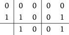
It is obvious that the first order IMEX-RK method is just taking the forward Euler discretization for the non-stiff term and the backward Euler discretization for the stiff term.

• Second order (two stages):

  

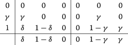
with $\gamma = 1 - \frac {\sqrt {2}}{2}$ and $\delta = 1 - \frac {1}{2\gamma }$.

• Third order (three stages):

  

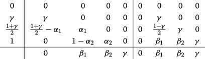
with γ the middle root of $6x^{3} - 18x^{2} + 9x - 1 = 0, \gamma \approx 0.435866521508459, \beta _{1} = -\frac {3}{2}\gamma ^{2} + 4\gamma -\frac {1}{4}, \beta _{2} = \frac {3}{2}\gamma ^{2} - 5 \gamma + \frac {5}{4}, \alpha _{1} = -0.35$ and $\alpha _{2} = \frac {\frac {1}{3} - 2\gamma ^{2} - 2\beta _{2}\alpha _{1}\gamma } {\gamma (1 - \gamma)}$.

4.2 Semi-discrete SDC discretizations

The SDC time discretization is based on the Picard integral equation and low order time integration methods, which are corrected iteratively, with the order of accuracy increased by one for each additional iteration. The key advantage of SDC method is that it can systematically and simply develop time integration methods of arbitrary high order of accuracy.

To define the semi-discrete SDC scheme, we further divide the time interval [t_n,t_n+1] into P subintervals by points t_n,m for m=0,1,⋯,P such that t_n=t_n,0<t_n,1<⋯<t_n,m<⋯<t_n,P=t_n+1. Let △t_n,m=t_n,m+1−t_n,m and $\mathbf {u}^{k}_{n, m}$ denote the k-th order approximation to u(t_n,m). We choose the points $\{t_{n, m}\}^{p}_{m = 0}$ as Gauss-Lobatto nodes on [t_n,t_n+1]. Then the algorithm to calculate (k+1)-th order accuracy numerical solution of (7) advanced from time t_n to t_n+1 is given in Algorithm 1, where $I^{m + 1}_{m}\left (\mathbf {F}_{N}\left (t, \mathbf {u}^{k}\right) + \mathbf {F}_{S}\left (t, \mathbf {u}^{k}\right)\right)$ is the integral of the P-th degree interpolating polynomial on the P+1 points $\left (t_{n, m}, \mathbf {F}_{N}\left (t_{n, m}, \mathbf {u}^{k}_{n, m}\right) + \mathbf {F}_{S}\left (t_{n, m}, \mathbf {u}^{k}_{n, m}\right)\right)_{m = 0}^{P}$ over the subinterval [t_n,m,t_n,m+1].

4.3 Fully discrete schemes

Finally, as the implementation of IMEX-RK and SDC time discretizations to the semi-discrete LDG scheme (5) and (6), we will present the fully discrete LDG schemes in the following for the NS equations. We only present the third-order fully discrete scheme here and the lower order fully discrete schemes can be deduced similarly.

• Third order IMEX-RK-LDG scheme

  The LDG scheme with the third order IMEX-RK time marching method is given as :

  $$\begin{array}{*{20}l} \left(\mathbf{U}_{h}^{n, 1}, \mathbf{V}\right)_{K} &= \left(\mathbf{U}_{h}^{n}, \mathbf{V}\right)_{K} + \gamma \triangle t_{n} \left(\left(\mathbf{F}_{h}^{n}, \nabla \mathbf{V}\right)_{K} - \left(\widehat{\mathbf{F}}^{n}, \mathbf{V}\right)_{\partial{K}} \right) \\ &\quad- \gamma \triangle t_{n} \left(\left(\mathbf{G}_{h}^{n, 1}, \nabla \mathbf{V}\right)_{K} - \left(\widehat{\mathbf{G}}^{n, 1} \mathbf{n}, \mathbf{V}\right)_{\partial{K}} \right), \end{array} $$

  (8a)
  $$\begin{array}{*{20}l} \left(\mathbf{U}_{h}^{n, 2}, \mathbf{V}\right)_{K} &= \left(\mathbf{U}_{h}^{n}, \mathbf{V}\right)_{K} + \left(\frac{1 + \gamma}{2} - \alpha_{1}\right) \triangle t_{n} \left(\left(\mathbf{F}_{h}^{n}, \nabla \mathbf{V}\right)_{K} - \left(\widehat{\mathbf{F}}^{n}, \mathbf{V}\right)_{\partial{K}} \right) \\ &\quad+ \alpha_{1} \triangle t_{n} \left(\left(\mathbf{F}_{h}^{n, 1}, \nabla \mathbf{V}\right)_{K} - \left(\widehat{\mathbf{F}}^{n, 1}, \mathbf{V}\right)_{\partial{K}} \right) \\ &\quad- \frac{1 - \gamma}{2} \triangle t_{n} \left(\left(\mathbf{G}_{h}^{n, 1}, \nabla \mathbf{V}\right)_{K} - \left(\widehat{\mathbf{G}}^{n, 1} \mathbf{n}, \mathbf{V}\right)_{\partial{K}} \right) \\ &\quad- \gamma \triangle t_{n} \left(\left(\mathbf{G}_{h}^{n, 2}, \nabla \mathbf{V}\right)_{K} - \left(\widehat{\mathbf{G}}^{n, 2} \mathbf{n}, \mathbf{V}\right)_{\partial{K}} \right), \end{array} $$

  (8b)
  $$\begin{array}{*{20}l} \left(\mathbf{U}_{h}^{n, 3}, \mathbf{V}\right)_{K} &= \left(\mathbf{U}_{h}^{n}, \mathbf{V}\right)_{K} + (1 - \alpha_{2}) \triangle t_{n} \left(\left(\mathbf{F}_{h}^{n, 1}, \nabla \mathbf{V}\right)_{K} - \left(\widehat{\mathbf{F}}^{n, 1}, \mathbf{V}\right)_{\partial{K}} \right) \\ &\quad+ \alpha_{2} \triangle t_{n} \left(\left(\mathbf{F}_{h}^{n, 2}, \nabla \mathbf{V}\right)_{K} - \left(\widehat{\mathbf{F}}^{n, 2}, \mathbf{V}\right)_{\partial{K}} \right) \\ &\quad- \beta_{1} \triangle t_{n} \left(\left(\mathbf{G}_{h}^{n, 1}, \nabla \mathbf{V}\right)_{K} - \left(\widehat{\mathbf{G}}^{n, 1} \mathbf{n}, \mathbf{V}\right)_{\partial{K}} \right) \\ &\quad- \beta_{2} \triangle t_{n} \left(\left(\mathbf{G}_{h}^{n, 2}, \nabla \mathbf{V}\right)_{K} - \left(\widehat{\mathbf{G}}^{n, 2} \mathbf{n}, \mathbf{V}\right)_{\partial{K}} \right) \\ &\quad- \gamma \triangle t_{n} \left(\left(\mathbf{G}_{h}^{n, 3}, \nabla \mathbf{V}\right)_{K} - \left(\widehat{\mathbf{G}}^{n, 3} \mathbf{n}, \mathbf{V}\right)_{\partial{K}} \right), \end{array} $$

  (8c)
  $$\begin{array}{*{20}l} \left(\mathbf{U}_{h}^{n + 1}, \mathbf{V}\right)_{K} &= \left(\mathbf{U}_{h}^{n}, \mathbf{V}\right)_{K} + \beta_{1} \triangle t_{n} \left(\left(\mathbf{F}_{h}^{n, 1}, \nabla \mathbf{V}\right)_{K} - \left(\widehat{\mathbf{F}}^{n, 1}, \mathbf{V}\right)_{\partial{K}} \right) \\ &\quad+ \beta_{2} \triangle t_{n} \left(\left(\mathbf{F}_{h}^{n, 2}, \nabla \mathbf{V}\right)_{K} - \left(\widehat{\mathbf{F}}^{n, 2}, \mathbf{V}\right)_{\partial{K}} \right) \\ &\quad+ \gamma \triangle t_{n} \left(\left(\mathbf{F}_{h}^{n, 3}, \nabla \mathbf{V}\right)_{K} - \left(\widehat{\mathbf{F}}^{n, 3}, \mathbf{V}\right)_{\partial{K}} \right) \\ &\quad- \beta_{1} \triangle t_{n} \left(\left(\mathbf{G}_{h}^{n, 1}, \nabla \mathbf{V}\right)_{K} - \left(\widehat{\mathbf{G}}^{n, 1} \mathbf{n}, \mathbf{V}\right)_{\partial{K}} \right) \\ &\quad- \beta_{2} \triangle t_{n} \left(\left(\mathbf{G}_{h}^{n, 2}, \nabla \mathbf{V}\right)_{K} - \left(\widehat{\mathbf{G}}^{n, 2} \mathbf{n}, \mathbf{V}\right)_{\partial{K}} \right) \\ &\quad- \gamma \triangle t_{n} \left(\left(\mathbf{G}_{h}^{n, 3}, \nabla \mathbf{V}\right)_{K} - \left(\widehat{\mathbf{G}}^{n, 3} \mathbf{n}, \mathbf{V}\right)_{\partial{K}} \right), \end{array} $$

  (8d)
  $$\begin{array}{*{20}l} &\left(\mathbf{z}_{h}^{n, l}, \boldsymbol{\sigma}\right)_{K} = -\left(\mathbf{u}_{h}^{n, l}, \nabla \cdot \boldsymbol{\sigma}\right)_{K} + \left(\widehat{\mathbf{u}}^{n, l}, \boldsymbol{\sigma} \mathbf{n}\right)_{\partial{K}}, \quad l = 1, 2, 3, \end{array} $$

  (9a)
  $$\begin{array}{*{20}l} &\left(\mathbf{q}_{h}^{n, l}, \mathbf{p}\right)_{K} = \kappa \left(T_{h}^{n, l}, \nabla \cdot \mathbf{p}\right)_{K} - \kappa \left(\widehat{T}^{n, l}, \mathbf{p} \cdot \mathbf{n}\right)_{\partial{K}}, \quad l = 1, 2, 3, \end{array} $$

  (9b)

  for any test function V∈V_h,σ∈Σ_h,p∈W_h, with $\mathbf {U}_{h}^{n, l} = \left (\rho _{h}^{n, l}, \mathbf {m}_{h}^{n, l}, E_{h}^{n, l}\right)^{T}, \mathbf {F}_{h}^{n, l} = \mathbf {F}\left (\mathbf {U}_{h}^{n, l}\right)$, $\mathbf {G}_{h}^{n, l} = \mathbf {G}\left (\mathbf {U}_{h}^{n, l}, \boldsymbol {\tau }_{h}^{n, l}, \mathbf {q}_{h}^{n, l}\right), l = 0, 1, 2, 3$, and

  $$\begin{array}{*{20}l} \mathbf{u}_{h}^{n, l} &= \frac{\mathbf{m}_{h}^{n, l}}{\rho_{h}^{n, l}}, \quad l = 0, 1, 2, 3, \end{array} $$

  (10a)
  $$\begin{array}{*{20}l} \boldsymbol{\tau}_{h}^{n, l} &= \frac{1}{Re_{\infty}} \left(\mathbf{z}_{h}^{n, l} + \left(\mathbf{z}_{h}^{n, l}\right)^{T} - \frac{2}{3} tr\left(\mathbf{z}_{h}^{n, l}\right) \mathbf{I} \right), \quad l = 1, 2, 3, \end{array} $$

  (10b)
  $$\begin{array}{*{20}l} \kappa T_{h}^{n, l} &= \frac{\gamma}{Re_{\infty} Pr}\left(\frac{E_{h}^{n, l}}{\rho_{h}^{n, l}} - \frac{1}{2}\left|\mathbf{u}_{h}^{n, l}\right|^{2} \right), \quad l = 1, 2, 3, \end{array} $$

  (10c)

  and notations ∗^n,0=∗ⁿ.

• High order SDC-LDG scheme

  The LDG scheme with high order SDC time marching method reads : for any test function V∈V_h, σ∈Σ_h,p∈W_h, the following first order approximation as well as successive correction equations are satisfied

  $$\begin{array}{*{20}l} {}\left((\mathbf{U}_{h})_{n, m + 1}^{1}, \mathbf{V}\right)_{K} &= \left((\mathbf{U}_{h})_{n, m}^{1}, \mathbf{V}\right)_{K} + \triangle t_{n, m} \left(\left((\mathbf{F}_{h})_{n, m}^{1}, \nabla \mathbf{V}\right)_{K} - \left(\widehat{\mathbf{F}}_{n, m}^{1}, \mathbf{V}\right)_{\partial{K}} \right) \\ &\quad- \triangle t_{n, m} \left(\left((\mathbf{G}_{h})_{n, m + 1}^{1}, \nabla \mathbf{V}\right)_{K} - \left(\widehat{\mathbf{G}}_{n, m + 1}^{1} \mathbf{n}, \mathbf{V}\right)_{\partial{K}} \right), \end{array} $$

  (11a)
  $$\begin{array}{*{20}l} {}\left((\mathbf{U}_{h})_{n, m + 1}^{k + 1}, \mathbf{V}\right)_{K} &= \left((\mathbf{U}_{h})_{n, m}^{k + 1}, \mathbf{V}\right)_{K} + \triangle t_{n, m} \left(\left((\mathbf{F}_{h})_{n, m}^{k + 1}, \nabla \mathbf{V}\right)_{K} - \left(\widehat{\mathbf{F}}_{n, m}^{k + 1}, \mathbf{V}\right)_{\partial{K}} \right) \\ &\quad- \triangle t_{n, m} \left(\left((\mathbf{F}_{h})_{n, m}^{k}, \nabla \mathbf{V}\right)_{K} - \left(\widehat{\mathbf{F}}_{n, m}^{k}, \mathbf{V}\right)_{\partial{K}} \right) \\ &\quad- \triangle t_{n, m} \left(\left((\mathbf{G}_{h})_{n, m + 1}^{k + 1}, \nabla \mathbf{V}\right)_{K} - \left(\widehat{\mathbf{G}}_{n, m + 1}^{k + 1} \mathbf{n}, \mathbf{V}\right)_{\partial{K}} \right) \\ &\quad+ \triangle t_{n, m} \left(\left((\mathbf{G}_{h})_{n, m + 1}^{k}, \nabla \mathbf{V}\right)_{K} - \left(\widehat{\mathbf{G}}_{n, m + 1}^{k} \mathbf{n}, \mathbf{V}\right)_{\partial{K}} \right) \\ &\quad+ I_{m}^{m + 1} \left(\left((\mathbf{F}_{h})^{k}, \nabla \mathbf{V}\right)_{K} - \left(\widehat{\mathbf{F}}^{k}, \mathbf{V}\right)_{\partial{K}} \right) \\ &\quad- I_{m}^{m + 1} \left(\left((\mathbf{G}_{h})^{k}, \nabla \mathbf{V}\right)_{K} - \left(\widehat{\mathbf{G}}^{k} \mathbf{n}, \mathbf{V}\right)_{\partial{K}} \right), \end{array} $$

  (11b)

  for m=0,⋯,P−1,k=1,⋯,K, and

  $$\begin{array}{*{20}l} &\left((\mathbf{z}_{h})_{n, m}^{k}, \boldsymbol{\sigma}\right)_{K} = -\left((\mathbf{u}_{h})_{n, m}^{k}, \nabla \cdot \boldsymbol{\sigma}\right)_{K} + \left(\widehat{\mathbf{u}}_{n, m}^{k}, \boldsymbol{\sigma} \mathbf{n}\right)_{\partial{K}}, \end{array} $$

  (12a)
  $$\begin{array}{*{20}l} &\left((\mathbf{q}_{h})_{n, m}^{k}, \mathbf{p}\right)_{K} = \kappa \left(\left((T_{h})_{n, m}^{k}, \nabla \cdot \mathbf{p}\right)_{K} - \left(\widehat{T}_{n, m}^{k}, \mathbf{p} \cdot \mathbf{n}\right)_{\partial{K}} \right), \end{array} $$

  (12b)

  for m=0,⋯,P,k=1,⋯,K+1, where $(\mathbf {U}_{h})_{n, m}^{k} = \left ((\rho _{h})_{n, m}^{k}, (\mathbf {m}_{h})_{n, m}^{k}, (E_{h})_{n, m}^{k}\right)^{T}$, $(\mathbf {F}_{h})_{n, m}^{k} = \mathbf {F}\left ((\mathbf {U}_{h})_{n, m}^{k}\right)$, $(\mathbf {G}_{h})_{n, m}^{k} = \mathbf {G}\left ((\mathbf {U}_{h})_{n, m}^{k}, (\boldsymbol {\tau }_{h})_{n, m}^{k}, (\mathbf {q}_{h})_{n, m}^{k}\right)$ and

  $$\begin{array}{*{20}l} (\mathbf{u}_{h})_{n, m}^{k} &= \frac{(\mathbf{m}_{h})_{n, m}^{k}}{(\rho_{h})_{n, m}^{k}}, \end{array} $$

  (13a)
  $$\begin{array}{*{20}l} (\boldsymbol{\tau}_{h})_{n, m}^{k} &= \frac{1}{Re_{\infty}} \left((\mathbf{z}_{h})_{n, m}^{k} + \left((\mathbf{z}_{h})_{n, m}^{k}\right)^{T} - \frac{2}{3} tr\left((\mathbf{z}_{h})_{n, m}^{k}\right) \mathbf{I} \right), \end{array} $$

  (13b)
  $$\begin{array}{*{20}l} \kappa (T_{h})_{n, m}^{k} &= \frac{\gamma}{Re_{\infty} Pr} \left(\frac{(E_{h})_{n, m}^{k}}{(\rho_{h})_{n, m}^{k}} - \frac{1}{2} \left|(\mathbf{u}_{h})_{n, m}^{k}\right|^{2} \right), \end{array} $$

  (13c)

  for m=0,⋯,P,k=1,⋯,K+1.

  Finally we can obtain the (K+1)-th approximation $\mathbf {U}_{h}^{n + 1} = (\mathbf {U}_{h})_{n, P}^{K + 1}$ at time t_n+1.

5 Mesh adaptation

In this section, we mainly present the detailed implementation of the h-adaptation algorithm for the structured mesh consisting of quadrilateral elements in 2D or hexahedral elements in 3D, including the method to refine and coarsen elements, the criteria to select candidate elements for refinement and coarsening, and the specific procedure of mesh adaptation.

5.1 Refinement and coarsening of elements

For the data structure of adaptive mesh, we adopt a generalized binary tree, i.e., quadtree in 2D and octree in 3D, to store all the elements, that is, a parent element is always divided into 4 in 2D or 8 in 3D child elements. The DG method is extremely local in data communication and allows the appearance of hanging nodes. This means that an element can be refined an unlimited number of times, regardless of its immediate neighbors. However, if a huge difference between the levels of adjacent elements exists, the stability of the resulting numerical scheme will be damaged. In order to enhance the mesh quality and the stability of the scheme, we impose the quadtree or octree balanced, that is, the levels between two adjacent elements differ at most by 1.

The numerical solution U_h restricted in element K can be expressed as

$$ \mathbf{U}_{h}(\mathbf{x}, t)|_{K} = \sum_{l = 1}^{N_{b}} \mathbf{U}_{l}^{K}(t) v_{l}^{K}(\mathbf{x}), $$

(14)

where $\mathbf {U}_{l}^{K}(t)$ and $v_{l}^{K}(\mathbf {x}), l = 1, \cdots, N_{b}$ denote the degrees of freedom and basis functions, respectively, in element K. To maintain the accuracy and local conservation of the solutions, we adopt L² projection to obtain the degrees of freedom in the new generated elements during refinement and coarsening. In detail, provided the numerical solution U_h is already known on the mesh $\mathcal {T}_{h}(t_{n})$, we require to determine the degrees of freedom $\mathbf {U}_{l}^{K'}(t_{n}), l = 1, \cdots, N_{b}$ in the new element $K' \in \mathcal {T}_{h}(t_{n + 1})$. Let Uh′ be the L² projection of U_h, which is computed through the following equations:

$$ \int_{K'} \mathbf{U}'_{h}|_{K'} v_{l}^{K'}(\mathbf{x}) d\mathbf{x} = \int_{K'} \mathbf{U}_{h} v_{l}^{K'}(\mathbf{x}) d\mathbf{x}, \quad l = 1, \cdots, N_{b}. $$

(15)

Then the degrees of freedom $\mathbf {U}_{l}^{K'}(t_{n}), l = 1, \cdots, N_{b}$ can be obtained by substituting (14) into (15).

5.2 Indicators

A criterion will be presented to initially determine the candidate elements for refinement and coarsening in a given mesh. According to [16, 17], the gradient of density finds shock and contact discontinuity well, the divergence of velocity is direction independent and very effective in locating shock including strong shock and weak shock and the curl of velocity is also direction independent and very effective in finding shear and vortex. For these three different indicators, we compute the following quantities respectively:

$$ \eta_{gi} = |\nabla \rho|d_{i}^{\frac{3}{2}}, \quad \eta_{di} = |\nabla \cdot \mathbf{u}|d_{i}^{\frac{3}{2}}, \quad \eta_{ci} = |\nabla \times \mathbf{u}|d_{i}^{\frac{3}{2}}, \quad i = 1, \cdots, N_{c}, $$

where N_c is the total number of elements, $d_{i} = \sqrt {|K|}$ or $d_{i} = \sqrt [3]{|K|}$ depending on the dimension. The standard deviation of the gradient of density, the divergence and the curl of velocity are

$$ \eta_{g} = \sqrt{\frac{\sum_{i = 1}^{N_{c}} \eta_{gi}^{2}}{N_{c}}}, \quad \eta_{d} = \sqrt{\frac{\sum_{i = 1}^{N_{c}} \eta_{di}^{2}}{N_{c}}}, \quad \eta_{c} = \sqrt{\frac{\sum_{i = 1}^{N_{c}} \eta_{ci}^{2}}{N_{c}}}, $$

respectively. In our work, a single indicator or a combination of two of the above indicators will be taken into account for different problems. Suppose the level of all the elements in the initial mesh equals zero, and each element in the initial mesh can be refined at most LEV times. Based on the values of indicators, if only a single indicator, e.g., η_gi is considered, then

• If η_gi>ω₁η_g and the level of K <LEV, then K is marked as a candidate element for refinement,

• If η_gi<ω₂η_g and the level of K > 0, then K is marked as a candidate element for coarsening,

with problem dependent parameters ω_l,l=1,2. If a combination of two indicators, e.g., η_gi and η_di are employed, then

• If η_gi>ω₁η_g or η_di>ω₃η_d, and the level of K <LEV, then K is marked as a candidate element for refinement,

• If η_gi<ω₂η_g and η_di<ω₄η_d, and the level of K > 0, then K is marked as a candidate element for coarsening,

with problem dependent parameters ω_l,l=1,2,3,4. In general, ω₁ and ω₃ are chosen between 1.1 and 1.5, ω₂ and ω₄ are chosen between 0.1 and 0.5.

5.3 Strategy for refinement and coarsening

In the above subsection, several candidate elements for refinement and coarsening are selected through given criteria. And whether these elements can be ultimately refined or coarsened, they also have to adhere to the principle that the level difference between two adjacent elements is at most 1 to improve the stability and accuracy of the LDG methods. To satisfy this principle, we adopt the strategy “refinement must, coarsening can” in [15], which means that a candidate element flagged for refinement is certainly to be refined, and in comparison, a candidate element marked for coarsening may not be coarsened.

After the execution of Algorithm 2 and Algorithm 3 in sequence, we can obtain two sets C_r and C_c which contain the final elements for refinement and coarsening, respectively. In Algorithm 2, all the candidate elements for refinement will be refined, and some neighbors of these elements are also added to the set C_r to ensure the mesh quality. In Algorithm 3, a candidate element for coarsening may be deleted from the set C_c due to either the absence of marked for coarsening for its brother elements, or the level difference with its neighbors.

5.4 Flow chart for mesh adaptation

As an end of this section, we present the general procedure for the adaptive LDG methods. Given the initial coarse mesh $\mathcal {T}_{h}(t_{0})$ and final computational time T,

• Step 1 Initialize the level of all the elements in $\mathcal {T}_{h}(t_{0})$ to be 0 and obtain the degrees of freedom in each element $\left \{\mathbf {U}_{l}^{K}(t_{0}), \ l = 1, \cdots, N_{b}, \ K \in \mathcal {T}_{h}(t_{0})\right \}$ through L² projection for the initial exact solution.

• Step 2 Given the mesh $\mathcal {T}_{h}(t_{n})$ and the degrees of freedom in each element $\left \{\mathbf {U}_{l}^{K}(t_{n}), \ l = 1, \cdots, N_{b}, \ K \in \mathcal {T}_{h}(t_{n})\right \}$, an updated mesh $\mathcal {T}_{h}(t_{n + 1})$ is gained as follows:

  • Identify the candidate elements for refinement and coarsening in $\mathcal {T}_{h}(t_{n})$ through criteria in subsection 5.2.

  • Determine the final element sets C_r and C_c for refinement and coarsening through Algorithm 2 and Algorithm 3, respectively and subsequently.

  • For each element in C_r, divide it into 4 in 2D or 8 in 3D child elements, get the degrees of freedom of child elements by use of L² projection, and increase the level of child elements by one.

  • For child elements with the same parent element in C_c, delete them and get the degrees of freedom of the parent element through L² projection.

• Step 3 Obtain $\left \{\mathbf {U}_{l}^{K}(t_{n} + 1), \ l = 1, \cdots, N_{b}, \ K \in \mathcal {T}_{h}(t_{n} + 1)\right \}$ by aid of the LDG method coupled with an IMEX-RK or SDC method.

• Step 4 If t_n+1<T, go to Step 2.

6 Numerical experiments

In this section, we will carry out several numerical experiments including accuracy tests and other benchmark problems for the NS equations to evaluate the performance of the h-adaptive LDG methods. In addition, IMEX-RK and/or SDC time integration methods are adopted to solve the ODEs resulting from the spatial discretizations. Note, at every stage for the evolution in time, GMRES solver without any preconditioner is adopted to solve the two successive linear systems with respect to momentum and energy equations. In all experiments, the time step △t_n at time t_n is chosen to satisfy the following CFL condition

$$ \frac{d \triangle t_{n}}{\min_{K} h_{K}}\max_{K}(|\mathbf{u}_{K}| + a_{K}) < cfl, $$

where d≤3 denotes the dimension, h_K is the diameter of element K, u_K and a_K are the velocity vector and speed of sound at element K, respectively, cfl is the CFL number taken as 0.98, 0.3, 0.18 for the first, second and third order time discretizations, respectively. In the following simulations, unless otherwise stated, an element in a mesh will be refined at most LEV=3 times, that is, the depth of the generalized binary tree is 3.

Example 1

Accuracy test in two dimension

In order to demonstrate the uniform high order accuracy both in space and time of our proposed h-adaptive LDG scheme in conjunction with IMEX-RK or SDC methods, for the first test case we consider a smooth exact solution

$$\begin{array}{*{20}l} \rho(\mathbf{x}, t) &= 0.6 + 0.1 \sin(5 \pi t) \cos(2 \pi x) \cos(2 \pi y), \\ u(\mathbf{x}, t) &= \sin(3 \pi t) \sin(2 \pi x) \sin(2 \pi y), \\ v(\mathbf{x}, t) &= \sin(3 \pi t) \sin(4 \pi x) \sin(4 \pi y), \\ p(\mathbf{x}, t) &= 0.8 + 0.1 \sin(\pi t) \sin(2 \pi x) \cos(2 \pi y), \end{array} $$

(16)

for the compressible NS Eqs. (1) with d=2 and an additional source term, which is acquired by inserting (16) into (1). Additionally, we take the computational domain as [0,1]² with periodic boundary conditions and Reynolds number Re_∞=200,1000,5000, respectively. All the simulations are performed until time T=0.1 on a set of successively globally refined background meshes containing N×N,N=16,32,64,128 quadrilateral elements, respectively. For a fixed N×N background mesh, we randomly choose 2N candidate elements marked for refinement and the remaining elements marked for coarsening at each time step, and gain the final element sets C_r and C_c through Algorithms 2 and 3. The initial 16×16 background mesh and the adaptive mesh at some time based on the 32×32 background mesh are shown in Fig. 2. We adopt (k+1)-th order IMEX-RK or SDC time marching methods when k-th degree polynomials are employed. The L² errors and orders of accuracy of density, velocity and pressure for both two schemes are presented in Tables 1 and 2, respectively, which illustrate that our two schemes can both obtain the expected optimal order of accuracy for these physical quantities with various Reynolds numbers. Moreover, by comparing the results in Tables 1 and 2, we can conclude that the IMEX-RK and SDC methods with the same order share nearly identical accuracy based on the background meshes with the same number of elements. For further efficiency comparison between IMEX-RK and SDC methods, we run the simulations on the uniform 64×64 mesh to eliminate the influence of frequent mesh refinement and coarsening. It can be seen from Table 3 that, compared with the IMEX-RK scheme, the SDC time discretization takes nearly the same time for the second order case and twice the time for the third order case, respectively. This can evidently be explained by their respective number of stages (there are 2 stages for both the second order IMEX-RK and SDC schemes, 3 stages for the third order IMEX-RK scheme and 6 stages for the third order SDC scheme). However, unlike the IMEX-RK scheme, the SDC method of arbitrary high order of accuracy can be systematically and simply developed.

Fig. 2

Sample mesh for accuracy test in two dimension

Table 1 Accuracy test for adaptive IMEX-RK-LDG scheme of 2D NS equations

Table 2 Accuracy test for adaptive SDC-LDG scheme of 2D NS equations

Table 3 Simulation CPU time(s) of IMEX-RK and SDC methods based on the uniform 64×64 mesh

Example 2

Accuracy test in three dimension

In this example, we extend our accuracy test to three dimension, which is much more challenging to implement the procedure of refinement and coarsening for a general hexahedral mesh. To this end, similar to the two dimensional counterpart, an artificial exact smooth solution

$$\begin{array}{*{20}l} \rho(\mathbf{x}, t) &= 2 + 0.5e^{-t} \sin(2 \pi x) \sin(2 \pi y) \sin(2 \pi z), \\ u(\mathbf{x}, t) &= e^{-2t}\sin(2 \pi x) \cos(2 \pi y) \sin(2 \pi z), \\ v(\mathbf{x}, t) &= e^{-2t}\cos(2 \pi x) \sin(2 \pi y) \cos(2 \pi z), \\ w(\mathbf{x}, t) &= e^{-2t}\sin(2 \pi x) \sin(2 \pi y) \cos(2 \pi z), \\ p(\mathbf{x}, t) &= 1.5 + 0.2e^{-t}\cos(2 \pi x) \cos(2 \pi y) \cos(2 \pi z), \end{array} $$

(17)

is constructed to satisfy (1) with d=3 and an additional source term. We compute the numerical solution on [0,1]³ with periodic boundary conditions and Reynolds number Re_∞=200 till final time T=0.1. The series of background meshes are composed of N×N×N hexahedral elements with N=4,8,16,32, see Fig. 3 for the 3D adaptive sample mesh. We also compute the L² errors and orders of density, velocity and pressure for IMEX-RK-LDG and SDC-LDG schemes. As in the previous case, Tables 4 and 5 show that our adaptive methods can also achieve optimal order of accuracy for 3D NS equations and nearly the same accuracy is obtained for the two schemes with identical setup.

Fig. 3

Sample mesh for accuracy test in three dimension

Table 4 Accuracy test for adaptive IMEX-RK-LDG scheme of 3D NS equations

Table 5 Accuracy test for adaptive SDC-LDG scheme of 3D NS equations

Example 3

Efficiency test of h -adaptive methods

For the purpose of illustrating the superiority of the presented mesh adaptation technique compared with the uniform mesh method in terms of storage and computational time, we consider the evolution of an isentropic vortex in inviscid flows. This procedure is governed by the 2D Euler equations, which are obtained by neglecting the viscous effects and heat conduction, that is, omitting the right-hand side of Eqs. (1). The initial solution of this problem is obtained by adding some perturbations to the uniform mean flow ρ_∞=u_∞=v_∞=p_∞=1. The vortex perturbations of the temperature T, velocity field (u,v) and entropy S can be formulated as follows:

$$ \delta T = -\frac{(\gamma - 1)\epsilon^{2}}{8\gamma \pi^{2}}e^{1 - r^{2}}, \quad (\delta u, \delta v) = \frac{\epsilon}{2 \pi}e^{\frac{1 - r^{2}}{2}}(y_{0} - y, x - x_{0}), \quad \delta S = 0, $$

where r²=(x−x₀)²+(y−y₀)²,(x₀,y₀) is the coordinate of the vortex center and ε is the vortex strength. Then the initial solution is determined through isentropic relation

$$\begin{array}{*{20}l} \rho = (1 + \delta T)^{\frac{1}{\gamma - 1}}, \quad u = 1 + \delta u, \quad v = 1 + \delta v, \quad p = (1 + \delta T)^{\frac{\gamma}{\gamma - 1}}. \end{array} $$

The exact solution to this problem is simply the passive convection of the initial solution. We take (x₀,y₀)=(10,10),ε=5 and computational domain as [0,50]². The numerical solutions are computed using piecewise quadratic polynomials and third order SSP-RK method which is more suitable for hyperbolic conservation laws. For more details about SSP-RK methods, see [2–5]. To evaluate the efficiency improvement of the h-adaptive methods, we run the simulations both in uniform and adaptive meshes with Dirichlet boundary conditions till time T=0.1. For the adaptive case, a combination of indicators η_gi and η_ci with parameters ω₁=1.2,ω₂=0.3,ω₃=1.3 and ω₄=0.4 are employed, and the depth of the tree is LEV=4. The final adaptive mesh based on a 16×16 background mesh and the density distribution around the vortex are presented in Fig. 4. The computed L² errors of density as functions of the final number of elements in the mesh and CPU time are shown in Fig. 5, illustrating that the h-adaptive methods can use less degrees of freedom and CPU time when achieving the same L² error. Table 6 quantitatively shows that our h-adaptive methods can save 89.9% in storage and 70.4% in CPU time compared with the uniform mesh method when they achieve the same L² error 4.84E-6 of density.

Fig. 4

(a) The final adaptive mesh based on a 16×16 background mesh. (b) Density distribution around the vortex

Fig. 5

L² errors of density as functions of the final number of elements and CPU time(s) on uniform and adaptive meshes for the evolution of an isentropic vortex. (a) L² error versus #elements; (b) L² error versus CPU time(s)

Table 6 Comparison of uniform and adaptive meshes with respect to number of elements and CPU time(s) when achieving 4.84E-6 L² error of density for the evolution of an isentropic vortex

Example 4

Shock-tube problems

To explicitly show the shock-capturing property of our proposed methods, we simulate the Riemann problems which are usually taken as Euler benchmark problems directly using the NS equations. Specifically, the NS Eqs. (1) with d=1 and initial conditions

$$\mathbf{U}(x, 0) = \left\{\begin{array}{l} U_{L}, \quad x < 0, \\ U_{R}, \quad x > 0, \\ \end{array}\right. $$

are considered in this test case. We adopt the classical Sod and Lax initial settings:

$$\begin{array}{*{20}l} (\rho_{L}, u_{L}, p_{L}) = (1, 0, 1), \quad (\rho_{R}, u_{R}, p_{R}) = (0.125, 0, 0.1), \end{array} $$

(18)

and

$$\begin{array}{*{20}l} (\rho_{L}, u_{L}, p_{L}) = (0.445, 0.698, 3.528), \quad (\rho_{R}, u_{R}, p_{R}) = (0.125, 0, 0.1). \end{array} $$

(19)

We run the two simulations with Reynolds number Re_∞=1800,P² element, third order IMEX-RK methods as well as a combination of indicators η_gi and η_di with parameters ω₁=1.2,ω₂=0.3,ω₃=1.2, and ω₄=0.3 on a background mesh of 200 cells till time T=0.25 and T=0.13, respectively. Figures 6 and 7 show the comparisons of density, velocity, pressure, specific internal energy between the Euler exact solutions and the NS numerical solutions. Note, the points for the NS numerical solutions are plotted every four cells and more points are clustered near the shock waves, contact discontinuities and rarefaction waves due to mesh adaptation to get better resolution.

Fig. 6

Sod shock-tube problem, Re_∞=1800,P²

Fig. 7

Lax shock-tube problem, Re_∞=1800,P²

Example 5

Taylor-Green vortex

We consider the Taylor-Green vortex, which is a low Mach number problem, in this test case. The initial solution of this problem is

$$\begin{array}{*{20}l} \rho(\mathbf{x}, 0) &= 1, \\ u(\mathbf{x}, 0) &= \sin(x) \cos(y), \\ v(\mathbf{x}, 0) &= -\cos(x) \sin(y), \\ p(\mathbf{x}, 0) &= \frac{p_{0}}{\gamma - 1} + \frac{1}{4}(\cos(2x) + \cos(2y)), \end{array} $$

with p₀=10⁵. This configuration leads to a characteristic Mach number M≈1.7·10⁻³, thus corresponds to the low Mach number regime [27]. The computational domain is [0,2π]². We simulate this procedure on a 64×64 background mesh with periodic boundary conditions till final time T=0.1. The (k+1)-th order IMEX-RK time discretization will be employed when P^k element is used. A single adaptive indicator η_ci with parameters ω₁=1.5,ω₂=0.5 is adopted. As is shown in Fig. 8, the vortex can be accurately captured by the adaptive mesh, and the contours become smoother when higher order elements are employed.

Fig. 8

Taylor-Green vortex. Adaptive mesh and vorticity contours with 20 equally spaced contour lines from -1.998 to 1.998

Example 6

Subsonic flow around a NACA0012 airfoil

In this test case we consider a subsonic flow around a NACA0012 airfoil which is symmetric about the x-axis with upper and lower surfaces described by functions [34]

$$\begin{array}{*{20}l} y^{\pm}(x) = \pm 5 \times 0.12 \times (0.2969\sqrt{x} - 0.126x - 0.3516x^{2} + 0.2843x^{3} - 0.1015x^{4}), \\ 0 \leq x \leq 1. 008930411365, \end{array} $$

and we require to rescale y^± so as to gain an airfoil of unit chord length. A rather coarse 64×16 C-type background mesh which extends about 20 chord length away from the airfoil is adopted for computation, see Fig. 9 for an impression of the mesh. The subsonic flow has configuration of Mach number M_∞=0.5, angle of attack α=0^∘ and Reynolds number Re_∞=5000. We apply an adiabatic no-slip wall boundary condition along the airfoil, subsonic inflow and outflow boundary conditions at respective farfield boundaries. We employ also a combination of indicators η_gi and η_di with parameters ω₁=1.2,ω₂=0.3,ω₃=1.2, and ω₄=0.3. P² element as well as the first order IMEX-RK time discretization is used since this is a steady state simulation. The adaptive mesh and the computed Mach number contours are presented in Fig. 10, clearly showing that the elements along and behind the wake of the airfoil can be locally refined to capture the more complex flow field. The distribution of pressure coefficient along the airfoil wall is further displayed in Fig. 11 and is consistent with the results presented in [6, 10].

Fig. 9

Background mesh for NACA0012 airfoil

Fig. 10

(a) Adaptive mesh and (b) the contour plots corresponding to P² solution for subsonic flow around a NACA0012 airfoil, 30 equally spaced contour lines are used to plot Mach number from 0.025 to 0.580

Fig. 11

Pressure coefficient for subsonic flow around a NACA0012 airfoil

Example 7

Supersonic flow past a NACA0012 airfoil

In this test case, the profile of the airfoil and the initial background mesh remain the same as in the previous subsonic case. The supersonic flow with Mach number M_∞=2 passes through the computational domain at an angle of attack α=10^∘ and Reynolds number Re_∞=106. An adiabatic no-slip wall boundary condition is imposed on the airfoil and at the farfield part of the computational domain, supersonic/subsonic inflow and supersonic/subsonic outflow boundary conditions are assumed, respectively, based on the uniform freestream and the unit normal vectors to the outer boundary. A salient feature of this case is the formation of a bow shock in front of the profile. We will also apply a combination of indicators η_gi and η_di with parameters ω₁=1.2,ω₂=0.3,ω₃=1.2 and ω₄=0.3. Again owing to steady state simulation, P² element as well as the first order IMEX-RK time discretization is employed. Figure 12 shows the adaptive mesh, Mach number and pressure contours of the numerical solution. Evidently, the bow shock can be captured with a nice resolution by virtue of local grid refinement. The pressure distribution is also given in Fig. 13.

Fig. 12

(a) Adaptive mesh and the contour plots corresponding to P² solution for supersonic flow past a NACA0012 airfoil, 30 equally spaced contour lines are used to plot (b) Mach number from 0.15 to 2.15, and (c) pressure from 0.61 to 5.41

Fig. 13

Pressure coefficient for supersonic flow past a NACA0012 airfoil

Example 8

Rayleigh-Taylor instability

In order to show the capability of our methods to capture the small-scale features of complicated flow structures, we consider the Rayleigh-Taylor instability phenomenon, which usually occurs at an interface between two fluids with different densities when the acceleration is directed from the heavy fluid to the light fluid, see [35, 36] for a detailed description of this phenomenon. We take the computational domain as [0,0.25]×[0,1]. The initial solution is

$$ (\rho, u, v, p) = \left\{\begin{array}{l} (2, 0, -0.025a\cos(8\pi x), 1 + 2y), \quad y \in (0, 0.5), \\ (1, 0, -0.025a\cos(8\pi x), y + 1.5), \quad y \in [0.5, 1), \end{array}\right. $$

where $a = \sqrt {\frac {\gamma p}{\rho }}$ is the sound speed with ratio of specific heats $\gamma = \frac {5}{3}$. The Prandtl number is taken as Pr=0.7 for this test case. An adiabatic, reflective boundary condition is imposed for the left and right boundaries. At the bottom and top boundaries, the flow values are set as

$$ (\rho, u, v, p) = \left\{\begin{array}{l} (2, 0, 0, 1), \quad y = 0, \\ (1, 0, 0, 2.5), \quad y = 1, \end{array}\right. $$

respectively. The source term ρ is added to the right hand side of the second momentum equation and ρv is added to the right hand side of the energy equation in (1). All the simulations are based on a 30×120 background mesh till final time T=1.95, and the (k+1)-th order IMEX-RK time discretization will be employed when P^k element is used. For the NS simulations, we adopt a single indicator η_gi with parameters ω₁=1.5,ω₂=0.5. Computational results with Reynolds number 50000 and 150000 are shown in Figs. 14 and 15, respectively. As can be seen, the interface between two fluids with different densities becomes thinner as the Reynolds number increases. Our adaptive methods can capture the interface and small-scale features precisely, and the resolution of P² element can even be comparable to that obtained with the ninth-order WENO scheme on a 600×2400 uniform mesh in [36]. The adaptive meshes and density contours of the Euler simulations with TVB limiter [3] and without TVB limiter are also presented in Figs. 16 and 17 by using adaptive parameters ω₁=1.2,ω₂=0.3. Due to the absence of physical viscosities, there exist more small-scale flow structures in these simulations, and the resolution of P² element can be comparable to that obtained with the ninth-order WENO scheme on a 480×1920 uniform mesh in [35].

Fig. 14

NS simulations for Rayleigh-Taylor instability with Reynolds number Re_∞=50000. From left to right: adaptive mesh for P¹ element; 30 equally spaced density contours from 0.8728 to 2.2249 for P¹ element; adaptive mesh for P² element; 30 equally spaced density contours from 0.8733 to 2.2262 for P² element

Fig. 15

NS simulations for Rayleigh-Taylor instability with Reynolds number Re_∞=150000. From left to right: adaptive mesh for P¹ element; 30 equally spaced density contours from 0.8608 to 2.2316 for P¹ element; adaptive mesh for P² element; 30 equally spaced density contours from 0.8712 to 2.2301 for P² element

Fig. 16

Euler simulations for Rayleigh-Taylor instability with TVB limiter. From left to right: adaptive mesh for P¹ element; 30 equally spaced density contours from 0.8620 to 2.2407 for P¹ element; adaptive mesh for P² element; 30 equally spaced density contours from 0.8705 to 2.2362 for P² element

Fig. 17

Euler simulations for Rayleigh-Taylor instability without TVB limiter. From left to right: adaptive mesh for P¹ element; 30 equally spaced density contours from 0.6548 to 2.4582 for P¹ element; adaptive mesh for P² element; 30 equally spaced density contours from 0.6852 to 2.3728 for P² element

7 Conclusions

In this paper, we have presented an h-adaptive LDG method for the solution of the unsteady compressible NS equations. To achieve the uniform high order accuracy both in space and time, avoid the extremely small time step restriction of explicit methods as well as the construction of large Jacobian matrix in implicit methods, two semi-implicit time marching methods including the classical IMEX-RK methods and the SDC methods were also employed for temporal discretizations. In the process of mesh adaptation, indicators are computed in each element of the mesh based on the gradient of density, the divergence and curl of velocity field to pick candidate elements for refinement and coarsening. We also adopt the strategy of “refinement must, coarsening can” to determine the ultimate element lists for refinement and coarsening. These proposed methods have been successfully implemented in a sequence of numerical examples, illustrating their expected optimal order of convergence, efficiency and capabilities in flow problems. Due to the high order accuracy and easy implementation, the h-adaptive LDG methods coupled with IMEX-RK or SDC methods provide an appealing alternative for unsteady compressible NS equations which require to accurately capture the detailed flow structures at any time.

References

Reed WH, Hill TR (1973) Triangular mesh methods for the neutron transport equation. Tech Rep LA-UR-73-479. Los Alamos Scientific Lab, New Mexico.
Cockburn B, Hou S, Shu C-W (1990) The Runge-Kutta local projection discontinuous Galerkin finite element method for conservation laws. IV. The multidimensional case. Math Comput 54(190):545–581.
Cockburn B, Lin S-Y, Shu C-W (1989) TVB Runge-Kutta local projection discontinuous Galerkin finite element method for conservation laws III: one-dimensional systems. J Comput Phys 84(1):90–113.
Cockburn B, Shu C-W (1989) TVB Runge-Kutta local projection discontinuous Galerkin finite element method for conservation laws II. General framework. Math Comput 52(186):411–435.
Cockburn B, Shu C-W (1998) The Runge–Kutta discontinuous Galerkin method for conservation laws V: multidimensional systems. J Comput Phys 141(2):199–224.
Bassi F, Rebay S (1997) A high-order accurate discontinuous finite element method for the numerical solution of the compressible Navier–Stokes equations. J Comput Phys 131(2):267–279.
Bassi F, Crivellini A, Rebay S, Savini M (2005) Discontinuous Galerkin solution of the Reynolds-averaged Navier–Stokes and k– ω turbulence model equations. Comput Fluids 34(4-5):507–540.
Hartmann R, Houston P (2006) Symmetric interior penalty DG methods for the compressible Navier–Stokes equations II: Goal–oriented a posteriori error estimation. Int J Numer Anal Model 3(1):141–162.
Klaij CM, van der Vegt JJ, van der Ven H (2006) Space–time discontinuous Galerkin method for the compressible Navier–Stokes equations. J Comput Phys 217(2):589–611.
Luo H, Luo L, Nourgaliev R, Mousseau VA, Dinh N (2010) A reconstructed discontinuous Galerkin method for the compressible Navier–Stokes equations on arbitrary grids. J Comput Phys 229(19):6961–6978.
Liu H, Yan J (2009) The direct discontinuous Galerkin (DDG) methods for diffusion problems. SIAM J Numer Anal 47(1):675–698.
Cheng J, Yang X, Liu X, Liu T, Luo H (2016) A direct discontinuous Galerkin method for the compressible Navier–Stokes equations on arbitrary grids. J Comput Phys 327:484–502.
Cockburn B, Shu C-W (1998) The local discontinuous Galerkin method for time-dependent convection-diffusion systems. SIAM J Numer Anal 35(6):2440–2463.
Xu Y, Shu C-W (2010) Local discontinuous Galerkin methods for high-order time-dependent partial differential equations. Commun Comput Phys 7(1):1–46.
Tian L, Xu Y, Kuerten JG, van der Vegt JJ (2016) An h-adaptive local discontinuous Galerkin method for the Navier–Stokes–Korteweg equations. J Comput Phys 319:242–265.
Liu J, Qiu J, Goman M, Li X, Liu M (2016) Positivity-preserving Runge-Kutta discontinuous Galerkin method on adaptive Cartesian grid for strong moving shock. Numer Math Theory Methods Appl 9(1):87–110.
Liu J, Qiu J, Hu O, Zhao N, Goman M, Li X (2013) Adaptive Runge–Kutta discontinuous Galerkin method for complex geometry problems on Cartesian grid. Int J Numer Methods Fluids 73(10):847–868.
Pareschi L, Russo G (2005) Implicit–explicit Runge–Kutta schemes and applications to hyperbolic systems with relaxation. J Sci Comput 25(1):129–155.
Wang H, Shu C-W, Zhang Q (2016) Stability analysis and error estimates of local discontinuous Galerkin methods with implicit–explicit time-marching for nonlinear convection–diffusion problems. Appl Math Comput 272:237–258.
Wang H, Wang S, Zhang Q, Shu C-W (2016) Local discontinuous Galerkin methods with implicit-explicit time-marching for multi-dimensional convection-diffusion problems. ESAIM: Math Model Numer Anal 50(4):1083–1105.
Xia Y, Xu Y, Shu C-W (2007) Efficient time discretization for local discontinuous Galerkin methods. Discret Contin Dyn Syst-B 8(3):677–693.
Guo R, Filbet F, Xu Y (2016) Efficient high order semi-implicit time discretization and local discontinuous Galerkin methods for highly nonlinear PDEs. J Sci Comput 68(3):1029–1054.
Guo R, Xia Y, Xu Y (2017) Semi-implicit spectral deferred correction methods for highly nonlinear partial differential equations. J Comput Phys 338:269–284.
Boscarino S, Russo G, Scandurra L (2018) All Mach number second order semi-implicit scheme for the Euler equations of gas dynamics. J Sci Comput 77(2):850–884.
Boscheri W, Dimarco G, Loubère R, Tavelli M, Vignal M-H (2020) A second order all Mach number IMEX finite volume solver for the three dimensional Euler equations. J Comput Phys 415:109486.
Boscheri W, Pareschi L (2021) High order pressure-based semi-implicit IMEX schemes for the 3D Navier-Stokes equations at all Mach numbers. J Comput Phys 434:110206.
Busto S, Río-Martín L, Vázquez-Cendón ME, Dumbser M (2021) A semi-implicit hybrid finite volume/finite element scheme for all Mach number flows on staggered unstructured meshes. Appl Math Comput 402:126117.
Busto S, Tavelli M, Boscheri W, Dumbser M (2020) Efficient high order accurate staggered semi-implicit discontinuous Galerkin methods for natural convection problems. Comput Fluids 198:104399.
Fambri F, Dumbser M (2017) Semi-implicit discontinuous Galerkin methods for the incompressible Navier–Stokes equations on adaptive staggered Cartesian grids. Comput Methods Appl Mech Eng 324:170–203.
Tavelli M, Dumbser M (2017) A pressure-based semi-implicit space–time discontinuous Galerkin method on staggered unstructured meshes for the solution of the compressible Navier–Stokes equations at all Mach numbers. J Comput Phys 341:341–376.
Toro EF (2009) Riemann solvers and numerical methods for fluid dynamics: a practical introduction. Springer, Berlin, Heidelberg.
Ascher UM, Ruuth SJ, Spiteri RJ (1997) Implicit-explicit Runge-Kutta methods for time-dependent partial differential equations. Appl Numer Math 25(2-3):151–167.
Calvo M, De Frutos J, Novo J (2001) Linearly implicit Runge–Kutta methods for advection–reaction–diffusion equations. Appl Numer Math 37(4):535–549.
Bristeau MO, Glowinski R, Periaux J, Viviand H (1987) Numerical simulation of compressible Navier-Stokes flows: a GAMM workshop. Vieweg+Teubner Verlag, Braunschweig.
Shi J, Zhang Y-T, Shu C-W (2003) Resolution of high order WENO schemes for complicated flow structures. J Comput Phys 186(2):690–696.
Zhang Y-T, Shi J, Shu C-W, Zhou Y (2003) Numerical viscosity and resolution of high-order weighted essentially nonoscillatory schemes for compressible flows with high Reynolds numbers. Phys Rev E 68(4):046709.
Acknowledgements
Not applicable.
Funding
Research of Yan Xu is supported by the National Numerical Windtunnel Project NNW2019ZT4-B08, NSFC grant No. 12071455.
Author information
Authors and Affiliations
Contributions
Xiangyi Meng: Formal analysis, Investigation, Methodology, Software, Writing-original draft, Writing-review & editing. Yan Xu: Conceptualization, Methodology, Funding acquisition, Resources, Supervision, Writing-review & editing. The authors read and approved the final manuscript.
Corresponding author
Ethics declarations
Competing interests
The authors declare that they have no known competing financial interests or personal relationships that could have appeared to influence the work reported in this paper.
Additional information
Publisher’s Note
Springer Nature remains neutral with regard to jurisdictional claims in published maps and institutional affiliations.
Rights and permissions
Open Access This article is licensed under a Creative Commons Attribution 4.0 International License, which permits use, sharing, adaptation, distribution and reproduction in any medium or format, as long as you give appropriate credit to the original author(s) and the source, provide a link to the Creative Commons licence, and indicate if changes were made. The images or other third party material in this article are included in the article’s Creative Commons licence, unless indicated otherwise in a credit line to the material. If material is not included in the article’s Creative Commons licence and your intended use is not permitted by statutory regulation or exceeds the permitted use, you will need to obtain permission directly from the copyright holder. To view a copy of this licence, visit http://creativecommons.org/licenses/by/4.0/.
About this article
Cite this article
Meng, X., Xu, Y. Adaptive local discontinuous Galerkin methods with semi-implicit time discretizations for the Navier-Stokes equations. Adv. Aerodyn. 4, 22 (2022). https://doi.org/10.1186/s42774-022-00110-4
Received:
Accepted:
Published:
DOI: https://doi.org/10.1186/s42774-022-00110-4